Run Traffic Assignment

Assign traffic flows to network edges using either Path-Sized Logit (PSL) or All-or-Nothing (AoN) assignment methods.

Usage

run_assignment(
  graph_df,
  od_matrix_long,
  directed = FALSE,
  cost.column = "cost",
  method = c("PSL", "AoN"),
  beta = 1,
  ...,
  detour.max = 1.5,
  angle.max = 90,
  unique.cost = TRUE,
  npaths.max = Inf,
  dmat.max.size = 10000^2,
  return.extra = NULL,
  verbose = TRUE,
  nthreads = 1L
)

# S3 method for class 'flownet'
print(x, ...)

Arguments

graph_df

A data.frame with columns from, to, and optionally a cost column. Represents the network graph with edges between nodes.

od_matrix_long

A data.frame with columns from, to, and flow. Represents the origin-destination matrix in long format with flow values.

directed

Logical (default: FALSE). Whether the graph is directed.

cost.column

Character string (default: "cost") or numeric vector. Name of the cost column in graph_df, or a numeric vector of edge costs with length equal to nrow(graph_df). The cost values are used to compute shortest paths and determine route probabilities.

method

Character string (default: "PSL"). Assignment method:

• "PSL": Path-Sized Logit model considering multiple routes with overlap correction

• "AoN": All-or-Nothing assignment, assigns all flow to the shortest path (faster but no route alternatives)

beta

Numeric (default: 1). Path-sized logit parameter (beta_PSL). Only used for PSL method.

...

Additional arguments (currently ignored).

detour.max

Numeric (default: 1.5). Maximum detour factor for alternative routes (applied to shortest paths cost). Only used for PSL method. This is a key parameter controlling the execution time of the algorithm: considering more routes (higher detour.max) substantially increases computation time.

angle.max

Numeric (default: 90). Maximum detour angle (in degrees, two sided). Only used for PSL method. I.e., nodes not within this angle measured against a straight line from origin to destination node will not be considered for detours.

unique.cost

Logical (default: TRUE). Deduplicates paths based on the total cost prior to generating them. Only used for PSL method. Since multiple 'intermediate nodes' may be on the same path, there is likely a significant number of duplicate paths which this option removes.

npaths.max

Integer (default: Inf). Maximum number of paths to compute per OD-pair. Only used for PSL method. If the number of paths exceeds this number, a random sample will be taken from all but the shortest path.

dmat.max.size

Integer (default: 1e4^2). Maximum size of distance matrices (both shortest paths and geodesic) to precompute. If smaller than n_nodes^2, then the full matrix is precomputed. Otherwise, it is computed in chunks as needed, where each chunk has dmat.max.size elements. Only used for PSL method.

return.extra

Character vector specifying additional results to return. Use "all" to return all available extras for the selected method.

Option	PSL	AoN	Description
"graph"	Yes	Yes	The igraph graph object
"paths"	Yes	Yes	PSL: list of lists of edge indices (multiple routes per OD); AoN: list of edge index vectors (one path per OD)
"edges"	Yes	No	List of edge indices used for each OD pair
"counts"	Yes	Yes	PSL: list of edge visit counts per OD; AoN: integer vector of global edge traversal counts
"costs"	Yes	Yes	PSL: list of path costs per OD; AoN: numeric vector of shortest path costs
"weights"	Yes	No	List of path weights (probabilities) for each OD pair

verbose

Logical (default: TRUE). Show progress bar and intermediate steps completion status?

nthreads

Integer (default: 1L). Number of threads (daemons) to use for parallel processing with mirai. Should not exceed the number of logical processors.

x

An object of class flownet, typically returned by run_assignment.

Value

A list of class "flownet" containing:

• call - The function call

• final_flows - Numeric vector of assigned flows for each edge (same length as nrow(graph_df))

• od_pairs_used - Indices of OD pairs with valid flows

• Additional elements as specified in return.extra:

  • graph - The igraph graph object

  • paths - For PSL: list of lists of edge indices (multiple routes per OD pair); for AoN: list of edge index vectors (one shortest path per OD pair)

  • edges - List of edge indices used for each OD pair (PSL only)

  • edge_counts - For PSL: list of edge visit counts per OD pair; for AoN: integer vector of global edge traversal counts

  • path_costs - For PSL: list of path costs per OD pair; for AoN: numeric vector of shortest path costs

  • path_weights - List of path weights (probabilities) for each OD pair (PSL only)

Details

This function performs traffic assignment using one of two methods: All-or-Nothing (AoN) is fast but assigns all flow to a single shortest path; Path-Sized Logit (PSL) considers multiple routes with overlap correction for more realistic flow distribution.

All-or-Nothing (AoN) Method

A simple assignment method that assigns all flow from each OD pair to the single shortest path. This is much faster than PSL but does not consider route alternatives or overlaps. Parameters detour.max, angle.max, unique.cost, npaths.max, beta, and dmat.max.size are ignored for AoN.

Path-Sized Logit (PSL) Method

A more sophisticated assignment method that considers multiple alternative routes and accounts for route overlap when assigning flows. The PSL model adjusts choice probabilities based on how much each route overlaps with other alternatives, preventing overestimation of flow on shared segments. The beta parameter controls the sensitivity to overlap.

PSL Model Formulation

The probability \(P_k\) of choosing route \(k\) from the set of alternatives \(K\) is: $$P_k = \frac{e^{V_k}}{\sum_{j \in K} e^{V_j}}$$ where the utility \(V_k\) is defined as: $$V_k = -C_k + \beta_{PSL} \ln(PS_k)$$ Here \(C_k\) is the generalized cost of route \(k\), \(\beta_{PSL}\) is the path-size parameter (the beta argument), and \(PS_k\) is the path-size factor.

The path-size factor quantifies route uniqueness: $$PS_k = \frac{1}{C_k} \sum_{a \in \Gamma_k} \frac{c_a}{\delta_a}$$ where \(\Gamma_k\) is the set of edges in path \(k\), \(c_a\) is the cost of edge \(a\), and \(\delta_a\) is the number of alternative routes using edge \(a\).

If a path is unique (\(\delta_a = 1\) for all edges), then \(PS_k = 1\) and the model reduces to standard MNL. For overlapping routes, \(PS_k < 1\) and \(\ln(PS_k) < 0\), so a positive beta penalizes overlap. Higher beta values strengthen penalization; beta = 0 gives standard MNL behavior.

For more information about the PSL model consult some of the references below.

Route Enumeration Algorithm

For each origin-destination pair, the algorithm identifies alternative routes as follows:

1. Compute the shortest path cost from origin to destination. If sqrt(dmat.max.size) < N.nodes, the entire shortest-path-distance matrix is precomputed.

2. For each potential intermediate node, calculate the total cost of going origin -> intermediate -> destination (also using the distance matrix).

3. Keep only routes where total cost is within detour.max times the shortest path cost.

4. If angle.max is specified, filter to intermediate nodes that lie roughly in the direction of the destination (within the specified angle - see further details below). If sqrt(dmat.max.size) < N.nodes a geodesic-distance-matrix is precomputed for speedy calculations using the triangle equation.

5. If unique.cost = TRUE, remove duplicate routes based on total cost - as multiple intermediate nodes may yield exactly the same route.

6. (Optionally) use npaths.max to sample the remaining routes if still too many.

7. Compute the actual paths and filter out those with duplicate edges (where the intermediate node is approached and departed via the same edge).

This pre-selection using distance matrices speeds up route enumeration considerably by avoiding the computation of implausible paths.

Coordinate-Based Filtering

When angle.max is specified and graph_df contains coordinate columns (FX, FY, TX, TY), the function uses geographic distance calculations to restrict detours. Only intermediate nodes that are (a) closer to the origin than the destination is, and (b) within the specified angle from the origin-destination line are considered. This improves both computational efficiency and route realism by excluding geographically implausible detours.

References

Ben-Akiva, M., & Bierlaire, M. (1999). Discrete choice methods and their applications to short term travel decisions. In R. W. Hall (Ed.), Handbook of Transportation Science (pp. 5-33). Springer US. doi:10.1007/978-1-4615-5203-1_2

Cascetta, E. (2001). Transportation systems engineering: Theory and methods. Springer.

Ben-Akiva, M., & Lerman, S. R. (1985). Discrete choice analysis: Theory and application to travel demand. The MIT Press.

Ramming, M. S. (2002). Network knowledge and route choice (Doctoral dissertation). Massachusetts Institute of Technology.

Prato, C. G. (2009). Route choice modeling: Past, present and future research directions. Journal of Choice Modelling, 2(1), 65-100. doi:10.1016/S1755-5345(13)70005-8

AequilibiaE Python Documentation: https://www.aequilibrae.com/develop/python/route_choice/path_size_logit.html

See also

flownet-package

Examples

library(flownet)
library(collapse)
#> collapse 2.1.6, see ?`collapse-package` or ?`collapse-documentation`
#> 
#> Attaching package: ‘collapse’
#> The following object is masked from ‘package:stats’:
#> 
#>     D
library(sf)

# Load existing network edges (exclude proposed new links)
africa_net <- africa_network[!africa_network$add, ]

# Convert to graph (use atomic_elem to drop sf geometry, qDF for data.frame)
graph <- atomic_elem(africa_net) |> qDF()
nodes <- nodes_from_graph(graph, sf = TRUE)

# Map cities/ports to nearest network nodes
nearest_nodes <- nodes$node[st_nearest_feature(africa_cities_ports, nodes)]

# Simple gravity-based OD matrix
od_mat <- outer(africa_cities_ports$population, africa_cities_ports$population) / 1e12
dimnames(od_mat) <- list(nearest_nodes, nearest_nodes)
od_matrix_long <- melt_od_matrix(od_mat)

# Run Traffic Assignment (All-or-Nothing method)
result_aon <- run_assignment(graph, od_matrix_long, cost.column = "duration",
                             method = "AoN", return.extra = "all")
#> Created graph with 1379 nodes and 2344 edges...
#> 495 OD-pairs have zero or non-finite flow values and will be skipped...
print(result_aon)
#> FlowNet object
#> Call: run_assignment(graph_df = graph, od_matrix_long = od_matrix_long,      cost.column = "duration", method = "AoN", return.extra = "all") 
#> 
#> Number of nodes: 1379 
#> Number of edges: 2344 
#> Number of simulations/OD-pairs: 204714 
#> 
#> Average path length in edges (SD): 34.99213  (19.56615)
#> Average number of visits per edge (SD): 3056.049  (5875.129)
#> Average path cost (SD): 4345.631  (2253.376)
#> 
#> Final flows summary statistics:
#>      N  Ndist     Mean       SD  Min       Max  Skew   Kurt
#>   2344   2017  2187.89  4553.86    0  37250.26  3.49  18.49
#>   1%  5%   10%    25%     50%      75%   90%       95%       99%
#>    0   0  1.08  36.57  295.39  1662.86  7581  11386.38  20188.24
# \donttest{
# Run Traffic Assignment (Path-Sized Logit method)
# Note: PSL is slower but produces more realistic flow distribution
result_psl <- run_assignment(graph, od_matrix_long, cost.column = "duration",
                             method = "PSL", nthreads = 1L,
                             return.extra = c("edges", "counts", "costs", "weights"))
#> Created graph with 1379 nodes and 2344 edges...
#> Computed distance matrix of dimensions 1379 x 1379 ...
#> 495 OD-pairs have zero or non-finite flow values and will be skipped...
print(result_psl)
#> FlowNet object
#> Call: run_assignment(graph_df = graph, od_matrix_long = od_matrix_long,      cost.column = "duration", method = "PSL", return.extra = c("edges",          "counts", "costs", "weights"), nthreads = 1L) 
#> 
#> Number of edges: 2344 
#> Number of simulations/OD-pairs: 204714 
#> 
#> Average number of edges utilized per simulation (SD): 561.081  (435.3152)
#> Average number of visits per edge (SD): 11.62403  (23.3552)
#> Average path cost (SD): 5019.838  (554.6268)
#> Average path weight (SD): 0.0293314  (0.0879165)
#> 
#> Final flows summary statistics:
#>      N  Ndist     Mean       SD  Min       Max  Skew   Kurt
#>   2344   2259  2188.73  4541.72    0  37246.92  3.48  18.43
#>   1%    5%   10%    25%     50%      75%      90%       95%       99%
#>    0  0.05  1.62  39.28  301.48  1677.97  7573.77  11419.34  19460.79

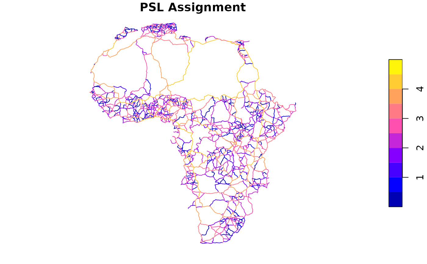
# Visualize AoN Results
africa_net$final_flows_log10 <- log10(result_psl$final_flows + 1)
plot(africa_net["final_flows_log10"], main = "PSL Assignment")

# }


# --- Trade Flow Disaggregation Example ---
# Disaggregate country-level trade to city-level using population shares

# Compute each city's share of its country's population
city_pop <- africa_cities_ports |> atomic_elem() |> qDF() |>
  fcompute(node = nearest_nodes,
           city = qF(city_country),
           pop_share = fsum(population, iso3, TRA = "/"),
           keep = "iso3")

# Aggregate trade to country-country level and disaggregate to cities
trade_agg <- africa_trade |> collap(quantity ~ iso3_o + iso3_d, fsum)
od_matrix_trade <- trade_agg |>
  join(city_pop |> add_stub("_o", FALSE), multiple = TRUE) |>
  join(city_pop |> add_stub("_d", FALSE), multiple = TRUE) |>
  fmutate(flow = quantity * pop_share_o * pop_share_d) |>
  frename(from = node_o, to = node_d) |>
  fsubset(flow > 0 & from != to)
#> left join: trade_agg[iso3_o] 1971/1971 (100%) <41.94:9.62> y[iso3_o] 452/453 (99.8%)
#> left join: x[iso3_d] 19685/19685 (100%) <418.83:9.62> y[iso3_d] 452/453 (99.8%)

# Run AoN assignment with trade flows
result_trade_aon <- run_assignment(graph, od_matrix_trade, cost.column = "duration",
                                   method = "AoN", return.extra = "all")
#> Created graph with 1379 nodes and 2344 edges...
print(result_trade_aon)
#> FlowNet object
#> Call: run_assignment(graph_df = graph, od_matrix_long = od_matrix_trade,      cost.column = "duration", method = "AoN", return.extra = "all") 
#> 
#> Number of nodes: 1379 
#> Number of edges: 2344 
#> Number of simulations/OD-pairs: 189020 
#> 
#> Average path length in edges (SD): 36.15387  (19.23456)
#> Average number of visits per edge (SD): 2915.445  (5685.838)
#> Average path cost (SD): 4477.602  (2187.799)
#> 
#> Final flows summary statistics:
#>      N  Ndist         Mean           SD  Min          Max  Skew   Kurt
#>   2344   1864  1'273306.07  2'915489.75    0  21'964576.8   3.7  18.51
#>   1%  5%  10%       25%        50%        75%          90%          95%
#>    0   0    0  17330.95  142839.71  911817.37  3'624008.55  6'948734.38
#>           99%
#>   14'969459.2
# \donttest{
# Visualize trade flow results
africa_net$trade_flows_log10 <- log10(result_trade_aon$final_flows + 1)
plot(africa_net["trade_flows_log10"], main = "Trade Flow Assignment (AoN)")


# Run PSL assignment with trade flows (nthreads can be increased for speed)
result_trade_psl <- run_assignment(graph, od_matrix_trade, cost.column = "duration",
                                   method = "PSL", nthreads = 1L,
                                   return.extra = c("edges", "counts", "costs", "weights"))
#> Created graph with 1379 nodes and 2344 edges...
#> Computed distance matrix of dimensions 1379 x 1379 ...
print(result_trade_psl)
#> FlowNet object
#> Call: run_assignment(graph_df = graph, od_matrix_long = od_matrix_trade,      cost.column = "duration", method = "PSL", return.extra = c("edges",          "counts", "costs", "weights"), nthreads = 1L) 
#> 
#> Number of edges: 2344 
#> Number of simulations/OD-pairs: 189020 
#> 
#> Average number of edges utilized per simulation (SD): 582.2353  (433.1455)
#> Average number of visits per edge (SD): 11.98732  (24.20449)
#> Average path cost (SD): 5171.393  (567.9297)
#> Average path weight (SD): 0.01955912  (0.07892114)
#> 
#> Final flows summary statistics:
#>      N  Ndist         Mean           SD  Min          Max  Skew   Kurt
#>   2344   2226  1'273430.15  2'909962.24    0  21'903042.7   3.7  18.53
#>   1%  5%    10%       25%        50%        75%          90%          95%
#>    0   0  71.23  17584.12  145086.78  908973.72  3'619965.69  6'948795.48
#>           99%
#>   14'978197.2

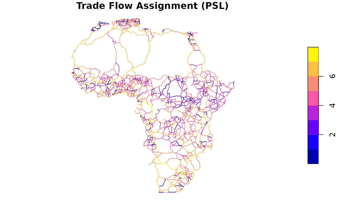
# Compare PSL vs AoN: PSL typically shows more distributed flows
africa_net$trade_flows_psl_log10 <- log10(result_trade_psl$final_flows + 1)
plot(africa_net["trade_flows_psl_log10"], main = "Trade Flow Assignment (PSL)")

# }