![]()
Introduction
collapse is a C/C++ based package for data transformation and statistical computing in R. It was first released on CRAN end of March 2020. The current version 1.3.1 is a mature piece of statistical software tested with > 7700 unit tests. collapse has 2 main aims:
To facilitate complex data transformation, exploration and computing tasks in R.
(In particular grouped and weighted statistical computations, advanced aggregation of multi-type data, advanced transformations of time series and panel data, and the manipulation of lists)
To help make R code fast, flexible, parsimonious and programmer friendly.
(Provide order of magnitude performance improvements via C/C++ and highly optimized R code, broad object orientation and attribute preservation, and a flexible programming infrastructure in standard and non-standard evaluation)
It is made compatible with dplyr, data.table and the plm approach to panel data. It can be installed in R using:
install.packages('collapse')

# See Documentation
help('collapse-documentation')
With this post I want to formally and briefly introduce collapse, provide a basic demonstration of important features, and end with a small benchmark comparing collapse to dplyr and data.table. I hope to convince that collapse provides a superior architecture for data manipulation and statistical computing in R, particularly in terms of flexibility, functionality, performance, and programmability.
Note: Please read this article here for better code appearance.
Demonstration
I start by briefly demonstrating the Fast Statistical Functions, which are a central feature of collapse. Currently there are 14 of them (fmean, fmedian, fmode, fsum, fprod, fsd, fvar, fmin, fmax, fnth, ffirst, flast, fNobs and fNdistinct), they are all S3 generic and support fast grouped and weighted computations on vectors, matrices, data frames, lists and grouped tibbles (class grouped_df). Calling these functions on different objects yields column-wise statistical computations:
library(collapse)
data("iris")            # iris dataset in base R
v <- iris$Sepal.Length  # Vector
d <- num_vars(iris)     # Saving numeric variables
g <- iris$Species       # Grouping variable (could also be a list of variables)

# Simple statistics
fmean(v)              # Vector
## [1] 5.843333
fsd(qM(d))            # Matrix (qM is a faster as.matrix)
## Sepal.Length  Sepal.Width Petal.Length  Petal.Width
##    0.8280661    0.4358663    1.7652982    0.7622377
fmode(d)              # Data frame
## Sepal.Length  Sepal.Width Petal.Length  Petal.Width
##          5.0          3.0          1.5          0.2

# Preserving data structure
fmean(qM(d), drop = FALSE)     # Still a matrix
##      Sepal.Length Sepal.Width Petal.Length Petal.Width
## [1,]     5.843333    3.057333        3.758    1.199333
fmax(d, drop = FALSE)          # Still a data.frame
##   Sepal.Length Sepal.Width Petal.Length Petal.Width
## 1          7.9         4.4          6.9         2.5
The functions fmean, fmedian, fmode, fnth, fsum, fprod, fvar and fsd additionally support weights1.
# Weighted statistics, similarly for vectors and matrices ...
wt <- abs(rnorm(fnrow(iris)))
fmedian(d, w = wt)
## Sepal.Length  Sepal.Width Petal.Length  Petal.Width
##          5.7          3.0          4.1          1.3
The second argument of these functions is called g and supports vectors or lists of grouping variables for grouped computations. For functions supporting weights, w is the third argument2.
# Grouped statistics
fmean(d, g)
##            Sepal.Length Sepal.Width Petal.Length Petal.Width
## setosa            5.006       3.428        1.462       0.246
## versicolor        5.936       2.770        4.260       1.326
## virginica         6.588       2.974        5.552       2.026

# Groupwise-weighted statistics
fmean(d, g, wt)
##            Sepal.Length Sepal.Width Petal.Length Petal.Width
## setosa         4.964652    3.389885     1.436666   0.2493647
## versicolor     5.924013    2.814171     4.255227   1.3273743
## virginica      6.630702    2.990253     5.601473   2.0724544

fmode(d, g, wt, ties = "max")  # Grouped & weighted maximum mode..
##            Sepal.Length Sepal.Width Petal.Length Petal.Width
## setosa              5.0           3          1.4         0.2
## versicolor          5.8           3          4.5         1.3
## virginica           6.3           3          5.1         2.3
Grouping becomes more efficient when factors or grouping objects are passed to g. Factors can efficiently be created using the function qF, and grouping objects are efficiently created with the function GRP3. As a final layer of complexity, all functions support transformations through the TRA argument.
library(magrittr)  # Pipe operators
# Simple Transformations
fnth(v, 0.9, TRA = "replace") %>% head   # Replacing values with the 90th percentile
## [1] 6.9 6.9 6.9 6.9 6.9 6.9
fsd(v, TRA = "/") %>% head               # Dividing by the overall standard-deviation (scaling)
## [1] 6.158928 5.917402 5.675875 5.555112 6.038165 6.521218

# Grouped transformations
fsd(v, g, TRA = "/") %>% head         # Grouped scaling
## [1] 14.46851 13.90112 13.33372 13.05003 14.18481 15.31960
fmin(v, g, TRA = "-") %>% head        # Setting the minimum value in each species to 0
## [1] 0.8 0.6 0.4 0.3 0.7 1.1
fsum(v, g, TRA = "%") %>% head        # Computing percentages
## [1] 2.037555 1.957651 1.877747 1.837795 1.997603 2.157411
ffirst(v, g, TRA = "%%") %>% head     # Taking modulus of first group-value, etc ...
## [1] 0.0 4.9 4.7 4.6 5.0 0.3

# Grouped and weighted transformations
fmedian(v, g, wt, "-") %>% head                      # Subtracting weighted group-medians
## [1]  0.1 -0.1 -0.3 -0.4  0.0  0.4
fmode(d, g, wt, "replace", ties = "min") %>% head(3) # replace with weighted minimum mode
##   Sepal.Length Sepal.Width Petal.Length Petal.Width
## 1            5           3          1.4         0.2
## 2            5           3          1.4         0.2
## 3            5           3          1.4         0.2
Currently there are 10 different replacing or sweeping operations supported by TRA, see ?TRA. TRA can also be called directly as a function which performs simple and grouped replacing and sweeping operations with computed statistics:
# Same as fmedian(v, TRA = "-")
TRA(v, median(v), "-") %>% head
## [1] -0.7 -0.9 -1.1 -1.2 -0.8 -0.4

# Replace values with 5% percentile by species
TRA(d, BY(d, g, quantile, 0.05), "replace", g) %>% head(3)
##   Sepal.Length Sepal.Width Petal.Length Petal.Width
## 1          4.4           3          1.2         0.1
## 2          4.4           3          1.2         0.1
## 3          4.4           3          1.2         0.1
The function BY is generic for Split-Apply-Combine computing with user-supplied functions. Another useful function is dapply (data-apply) for efficient column- and row-operations on matrices and data frames.
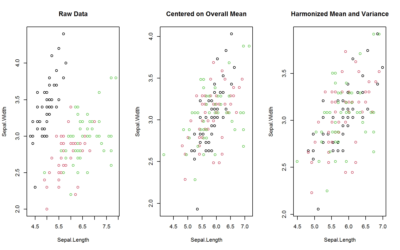
Some common panel data transformations like between- and (quasi-)within-transformations (averaging and centering using the mean) are implemented slightly more memory efficient in the functions fbetween and fwithin. The function fscale also exists for fast (grouped, weighted) scaling and centering (standardizing) and mean-preserving scaling. These functions provide further options for data harmonization, such as centering on the overall data mean or scaling to the within-group standard deviation4 (as shown below), as well as scaling / centering to arbitrary supplied means and standard deviations.
oldpar <- par(mfrow = c(1,3))
gv(d, 1:2) %>% {  # gv = shortcut for get_vars is > 2x faster than [.data.frame
plot(., col = g, main = "Raw Data")
plot(fwithin(., g, mean = "overall.mean"), col = g,
     main = "Centered on Overall Mean")
plot(fscale(., g, mean = "overall.mean", sd = "within.sd"), col = g,
     main = "Harmonized Mean and Variance")
}
par(oldpar)For the manipulation of time series and panel series, collapse offers the functions flag, fdiff and fgrowth.
# A sequence of lags and leads
flag(EuStockMarkets, -1:1) %>% head(3)
##       F1.DAX     DAX  L1.DAX F1.SMI    SMI L1.SMI F1.CAC    CAC L1.CAC F1.FTSE   FTSE L1.FTSE
## [1,] 1613.63 1628.75      NA 1688.5 1678.1     NA 1750.5 1772.8     NA  2460.2 2443.6      NA
## [2,] 1606.51 1613.63 1628.75 1678.6 1688.5 1678.1 1718.0 1750.5 1772.8  2448.2 2460.2  2443.6
## [3,] 1621.04 1606.51 1613.63 1684.1 1678.6 1688.5 1708.1 1718.0 1750.5  2470.4 2448.2  2460.2

# First and second annual difference of SAX and SMI indices (.c is for non-standard concatenation)
EuStockMarkets[, .c(DAX, SMI)] %>%
  fdiff(0:1 * frequency(.), 1:2) %>%
plot(main = c("DAX and SMI")) 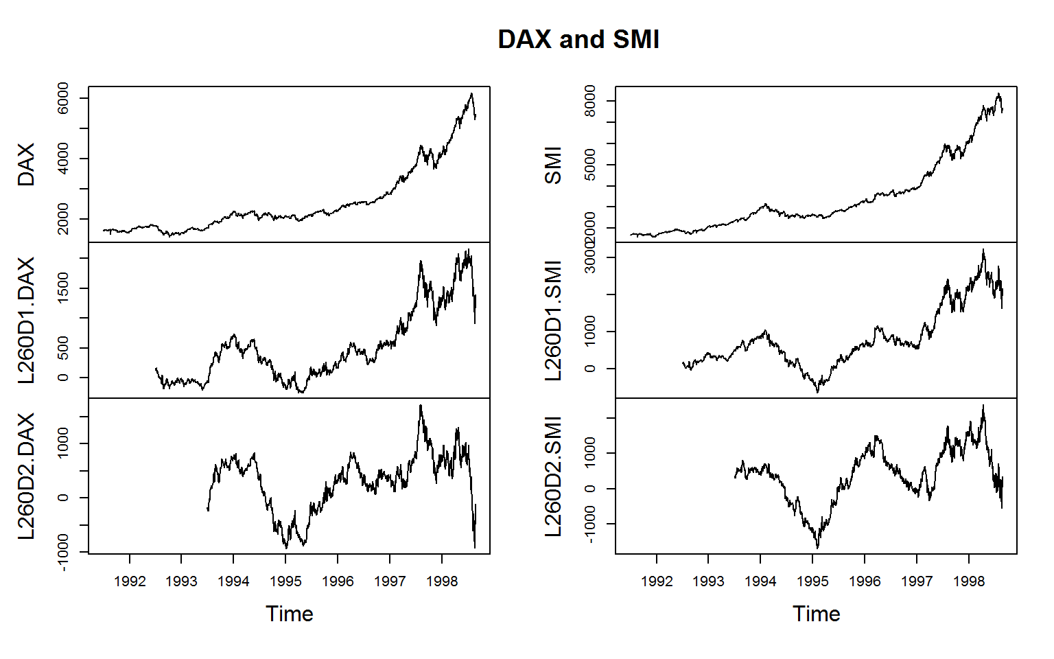
To facilitate programming and integration with dplyr, all functions introduced so far have a grouped_df method.
library(dplyr)
iris %>% add_vars(wt) %>%             # Adding weight vector to dataset
  filter(Sepal.Length < fmean(Sepal.Length)) %>%
  select(Species, Sepal.Width:wt) %>%
  group_by(Species) %>%               # Frequency-weighted group-variance, default (keep.w = TRUE)
  fvar(wt) %>% arrange(sum.wt)        # also saves group weights in a column called 'sum.wt'
## # A tibble: 3 x 5
##   Species    sum.wt Sepal.Width Petal.Length Petal.Width
##   <fct>       <dbl>       <dbl>        <dbl>       <dbl>
## 1 virginica    3.68      0.0193      0.00993      0.0281
## 2 versicolor  19.2       0.0802      0.181        0.0299
## 3 setosa      43.8       0.142       0.0281       0.0134
Since dplyr operations are rather slow, collapse provides its own set of manipulation verbs yielding significant performance gains.
# Same as above.. executes about 15x faster
iris %>% add_vars(wt) %>%
  fsubset(Sepal.Length < fmean(Sepal.Length),
          Species, Sepal.Width:wt) %>%
  fgroup_by(Species) %>%
  fvar(wt) %>% roworder(sum.wt)
## # A tibble: 3 x 5
##   Species    sum.wt Sepal.Width Petal.Length Petal.Width
##   <fct>       <dbl>       <dbl>        <dbl>       <dbl>
## 1 virginica    3.68      0.0193      0.00993      0.0281
## 2 versicolor  19.2       0.0802      0.181        0.0299
## 3 setosa      43.8       0.142       0.0281       0.0134

# Weighted demeaning
iris %>% fgroup_by(Species) %>% num_vars %>%
  fwithin(wt) %>% head(3)
## # A tibble: 3 x 4
##   Sepal.Length Sepal.Width Petal.Length Petal.Width
##          <dbl>       <dbl>        <dbl>       <dbl>
## 1       0.135        0.110      -0.0367     -0.0494
## 2      -0.0647      -0.390      -0.0367     -0.0494
## 3      -0.265       -0.190      -0.137      -0.0494

# Generate some additional logical data
settransform(iris,
  AWMSL = Sepal.Length > fmedian(Sepal.Length, w = wt),
  AGWMSL = Sepal.Length > fmedian(Sepal.Length, Species, wt, "replace"))

 # Grouped and weighted statistical mode
iris %>% fgroup_by(Species) %>% fmode(wt)
## # A tibble: 3 x 7
##   Species    Sepal.Length Sepal.Width Petal.Length Petal.Width AWMSL AGWMSL
##   <fct>             <dbl>       <dbl>        <dbl>       <dbl> <lgl> <lgl>
## 1 setosa              5             3          1.4         0.2 FALSE FALSE
## 2 versicolor          5.8           3          4.5         1.3 TRUE  FALSE
## 3 virginica           6.3           3          5.1         2.3 TRUE  FALSE
To take things a bit further, let’s consider some multilevel / panel data:
# World Bank World Development Data - supplied with collapse
head(wlddev, 3)
##       country iso3c       date year decade     region     income  OECD PCGDP LIFEEX GINI       ODA
## 1 Afghanistan   AFG 1961-01-01 1960   1960 South Asia Low income FALSE    NA 32.292   NA 114440000
## 2 Afghanistan   AFG 1962-01-01 1961   1960 South Asia Low income FALSE    NA 32.742   NA 233350000
## 3 Afghanistan   AFG 1963-01-01 1962   1960 South Asia Low income FALSE    NA 33.185   NA 114880000
All variables in this data have labels stored in a ‘label’ attribute (the default if you import from STATA / SPSS / SAS with haven). Variable labels can be accessed and set using vlabels and vlabels<-, and viewed together with names and classes using namlab. In general variable labels and other attributes will be preserved in when working with collapse. collapse provides some of the fastest and most advanced summary statistics:
# Fast distinct value count
fNdistinct(wlddev)
## country   iso3c    date    year  decade  region  income    OECD   PCGDP  LIFEEX    GINI     ODA
##     216     216      59      59       7       7       4       2    8995   10048     363    7564
# Use descr(wlddev) for a detailed description of each variable

# Checking for within-country variation
varying(wlddev, ~ iso3c)
## country    date    year  decade  region  income    OECD   PCGDP  LIFEEX    GINI     ODA
##   FALSE    TRUE    TRUE    TRUE   FALSE   FALSE   FALSE    TRUE    TRUE    TRUE    TRUE

# Panel data statistics: Summarize GDP and GINI overall, between and within countries
qsu(wlddev, pid = PCGDP + GINI ~ iso3c,
    vlabels = TRUE, higher = TRUE)
## , , PCGDP: GDP per capita (constant 2010 US$)
##
##              N/T        Mean          SD          Min         Max    Skew     Kurt
## Overall     8995  11563.6529  18348.4052     131.6464   191586.64  3.1121  16.9585
## Between      203  12488.8577  19628.3668     255.3999  141165.083   3.214  17.2533
## Within   44.3103  11563.6529   6334.9523  -30529.0928   75348.067   0.696  17.0534
##
## , , GINI: GINI index (World Bank estimate)
##
##             N/T     Mean      SD      Min      Max    Skew    Kurt
## Overall    1356  39.3976  9.6764     16.2     65.8  0.4613  2.2932
## Between     161  39.5799  8.3679  23.3667  61.7143  0.5169  2.6715
## Within   8.4224  39.3976  3.0406  23.9576  54.7976  0.1421  5.7781

# Panel data ACF: Efficient grouped standardizing and computing covariance with panel-lags
psacf(wlddev, ~ iso3c, ~ year, cols = 9:12)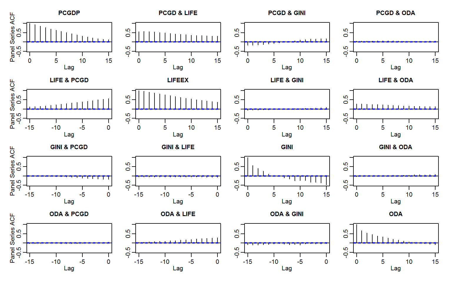
collapse also has its own very flexible data aggregation command called collap, providing fast and easy multi-data-type, multi-function, weighted, parallelized and fully customized data aggregation.
# Applying the mean to numeric and the mode to categorical data (first 2 arguments are 'by' and 'FUN')
collap(wlddev, ~ iso3c + decade, fmean,
       catFUN = fmode) %>% head(3)
##   country iso3c       date   year decade                     region      income  OECD PCGDP   LIFEEX
## 1   Aruba   ABW 1961-01-01 1962.5   1960 Latin America & Caribbean  High income FALSE    NA 66.58583
## 2   Aruba   ABW 1967-01-01 1970.0   1970 Latin America & Caribbean  High income FALSE    NA 69.14178
## 3   Aruba   ABW 1976-01-01 1980.0   1980 Latin America & Caribbean  High income FALSE    NA 72.17600
##   GINI      ODA
## 1   NA       NA
## 2   NA       NA
## 3   NA 33630000

# Same as a piped call..
wlddev %>% fgroup_by(iso3c, decade) %>%
  collapg(fmean, fmode) %>% head(3)
## # A tibble: 3 x 12
##   iso3c decade country date        year region             income    OECD  PCGDP LIFEEX  GINI     ODA
##   <fct>  <dbl> <chr>   <date>     <dbl> <fct>              <fct>     <lgl> <dbl>  <dbl> <dbl>   <dbl>
## 1 ABW     1960 Aruba   1961-01-01 1962. "Latin America & ~ High inc~ FALSE    NA   66.6    NA NA
## 2 ABW     1970 Aruba   1967-01-01 1970  "Latin America & ~ High inc~ FALSE    NA   69.1    NA NA
## 3 ABW     1980 Aruba   1976-01-01 1980  "Latin America & ~ High inc~ FALSE    NA   72.2    NA  3.36e7

# Same thing done manually... without column reordering
wlddev %>% fgroup_by(iso3c, decade) %>% {
  add_vars(fmode(cat_vars(.)),  # cat_vars selects non-numeric (categorical) columns
           fmean(num_vars(.), keep.group_vars = FALSE))
} %>% head(3)
## # A tibble: 3 x 12
##   iso3c decade country date       region             income    OECD   year PCGDP LIFEEX  GINI     ODA
##   <fct>  <dbl> <chr>   <date>     <fct>              <fct>     <lgl> <dbl> <dbl>  <dbl> <dbl>   <dbl>
## 1 ABW     1960 Aruba   1961-01-01 "Latin America & ~ High inc~ FALSE 1962.    NA   66.6    NA NA
## 2 ABW     1970 Aruba   1967-01-01 "Latin America & ~ High inc~ FALSE 1970     NA   69.1    NA NA
## 3 ABW     1980 Aruba   1976-01-01 "Latin America & ~ High inc~ FALSE 1980     NA   72.2    NA  3.36e7

# Adding weights: weighted mean and weighted mode (catFUN is 3rd argument)
wlddev$weights <- abs(rnorm(fnrow(wlddev)))
collap(wlddev, ~ iso3c + decade, fmean, fmode, # weights are also aggregated using sum
       w = ~ weights, wFUN = fsum) %>% head(3)
##   country iso3c       date     year decade                     region      income  OECD PCGDP
## 1   Aruba   ABW 1965-01-01 1963.375   1960 Latin America & Caribbean  High income FALSE    NA
## 2   Aruba   ABW 1967-01-01 1969.179   1970 Latin America & Caribbean  High income FALSE    NA
## 3   Aruba   ABW 1980-01-01 1980.443   1980 Latin America & Caribbean  High income FALSE    NA
##     LIFEEX GINI      ODA  weights
## 1 66.87902   NA       NA 4.527996
## 2 68.85522   NA       NA 7.314234
## 3 72.29649   NA 33630000 6.525710

# Can also apply multiple functions to columns, return in wide or long format or as list of data frames
collap(wlddev, PCGDP + LIFEEX ~ region + income,
       list(fmean, fsd, fmin, fmax), return = "long") %>% head(3)
##   Function              region              income     PCGDP   LIFEEX
## 1    fmean East Asia & Pacific         High income 26042.280 73.22799
## 2    fmean East Asia & Pacific Lower middle income  1621.178 58.83796
## 3    fmean East Asia & Pacific Upper middle income  3432.559 66.41750
The default (keep.col.order = TRUE) ensures that the data remains in the same order, and, when working with Fast Statistical Functions, all column attributes are preserved. When aggregating with multiple functions, you can parallelize over them (internally done with parallel::mclapply).
Time computations on panel data are also simple and computationally very fast.
# Panel Lag and lead of PCGDP and LIFEEX
L(wlddev, -1:1, PCGDP + LIFEEX ~ iso3c, ~year) %>% head3
##   iso3c year F1.PCGDP PCGDP L1.PCGDP F1.LIFEEX LIFEEX L1.LIFEEX
## 1   AFG 1960       NA    NA       NA    32.742 32.292        NA
## 2   AFG 1961       NA    NA       NA    33.185 32.742    32.292
## 3   AFG 1962       NA    NA       NA    33.624 33.185    32.742

# Equivalent piped call
wlddev %>% fgroup_by(iso3c) %>%
  fselect(iso3c, year, PCGDP, LIFEEX) %>%
  flag(-1:1, year) %>% head(3)
## # A tibble: 3 x 8
##   iso3c  year F1.PCGDP PCGDP L1.PCGDP F1.LIFEEX LIFEEX L1.LIFEEX
##   <fct> <int>    <dbl> <dbl>    <dbl>     <dbl>  <dbl>     <dbl>
## 1 AFG    1960       NA    NA       NA      32.7   32.3      NA
## 2 AFG    1961       NA    NA       NA      33.2   32.7      32.3
## 3 AFG    1962       NA    NA       NA      33.6   33.2      32.7

# Or using plm classes for panel data
pwlddev <- plm::pdata.frame(wlddev, index = .c(iso3c, year))
L(pwlddev, -1:1, cols = .c(PCGDP, LIFEEX)) %>% head(3)
##          iso3c year F1.PCGDP PCGDP L1.PCGDP F1.LIFEEX LIFEEX L1.LIFEEX
## ABW-1960   ABW 1960       NA    NA       NA    66.074 65.662        NA
## ABW-1961   ABW 1961       NA    NA       NA    66.444 66.074    65.662
## ABW-1962   ABW 1962       NA    NA       NA    66.787 66.444    66.074

# Growth rates in percentage terms: 1 and 10-year
G(pwlddev, c(1, 10), cols = 9:12) %>% head(3) # or use Dlog, or G(..., logdiff = TRUE) for percentages
##          iso3c year G1.PCGDP L10G1.PCGDP G1.LIFEEX L10G1.LIFEEX G1.GINI L10G1.GINI G1.ODA L10G1.ODA
## ABW-1960   ABW 1960       NA          NA        NA           NA      NA         NA     NA        NA
## ABW-1961   ABW 1961       NA          NA 0.6274558           NA      NA         NA     NA        NA
## ABW-1962   ABW 1962       NA          NA 0.5599782           NA      NA         NA     NA        NA
Equivalently we can can compute lagged / leaded and suitably iterated (log-) differences, as well as quasi-(log-)differences of the form \(x_t - \rho x_{t-1}\). The operators L, D, Dlog and G are shorthand’s for the functions flag, fdiff and fgrowth allowing formula input. Similar operators exist for fwithin, fscale, etc. which also support plm classes.
This short demonstration illustrated some basic features of collapse. A more complete overview of the package is provided in the documentation and the vignettes.
Benchmark
For benchmarking I use some product-level trade data from the UN Comtrade database, processed by tadestatistics.io.
library(tradestatistics)
# US HS4-level trade from 2000 to 2018
us_trade <- ots_create_tidy_data(years = 2000:2018,
                                 reporters = "usa",
                                 table = "yrpc")
Downloading US product-level trade (HS4) from 2000 to 2018 gives about 2.6 million observations:
fdim(us_trade)
## [1] 2569787      16
head(us_trade, 1)
##    year reporter_iso                                                   reporter_fullname_english
## 1: 2017          usa USA, Puerto Rico and US Virgin Islands (excludes Virgin Islands until 1981)
##    partner_iso partner_fullname_english section_code section_color section_shortname_english
## 1:         afg              Afghanistan           01       #74c0e2           Animal Products
##         section_fullname_english group_code group_fullname_english product_code
## 1: Live Animals; Animal Products         01          Animals; live         0101
##    product_shortname_english               product_fullname_english export_value_usd
## 1:                    Horses Horses, asses, mules and hinnies; live             3005
##    import_value_usd
## 1:               NA

# 19 years, 221 trading partners, 1222 products, unbalanced panel with product-time gaps...
fNdistinct(us_trade)
##                      year              reporter_iso reporter_fullname_english
##                        19                         1                         1
##               partner_iso  partner_fullname_english              section_code
##                       221                       221                        22
##             section_color section_shortname_english  section_fullname_english
##                        22                        22                        22
##                group_code    group_fullname_english              product_code
##                        97                        97                      1222
## product_shortname_english  product_fullname_english          export_value_usd
##                      1217                      1222                   1081492
##          import_value_usd
##                    684781

# Summarizing data between and within partner-product pairs
qsu(us_trade, pid = export_value_usd + import_value_usd ~ partner_iso + product_code)
## , , export_value_usd
##
##               N/T         Mean           SD              Min             Max
## Overall  2,450301  11,054800.6   157,295999                1  2.83030606e+10
## Between    205513  7,268011.31   118,709845                1  1.66436161e+10
## Within    11.9229  11,054800.6  68,344396.5  -1.01599067e+10  1.67185229e+10
##
## , , import_value_usd
##
##               N/T         Mean          SD              Min             Max
## Overall  1,248201  31,421502.4  505,644905                1  8.51970855e+10
## Between    130114  16,250758.2  328,538895                1  4.36545695e+10
## Within     9.5931  31,421502.4  212,076350  -3.32316111e+10  4.15739375e+10
It would also be interesting to summarize the trade flows for each partner, but that would be too large to print to the console. We can however get the qsu output as a list of matrices:
# Doing all of that by partner - variance of flows between and within traded products for each partner
l <- qsu(us_trade,
         by = export_value_usd + import_value_usd ~ partner_iso,
         pid = ~ partner_iso + product_code, array = FALSE)
str(l, give.attr = FALSE)
## List of 2
##  $ export_value_usd:List of 3
##   ..$ Overall: 'qsu' num [1:221, 1:5] 7250 12427 6692 5941 4017 ...
##   ..$ Between: 'qsu' num [1:221, 1:5] 901 1151 872 903 695 ...
##   ..$ Within : 'qsu' num [1:221, 1:5] 8.05 10.8 7.67 6.58 5.78 ...
##  $ import_value_usd:List of 3
##   ..$ Overall: 'qsu' num [1:221, 1:5] 1157 1547 361 1512 685 ...
##   ..$ Between: 'qsu' num [1:221, 1:5] 312 532 167 347 235 ...
##   ..$ Within : 'qsu' num [1:221, 1:5] 3.71 2.91 2.16 4.36 2.91 ...
Now with the function unlist2d, we can efficiently turn this into a tidy data frame:
unlist2d(l, idcols = c("Variable", "Trans"),
         row.names = "Partner", DT = TRUE) %>% head(3)
##            Variable   Trans Partner     N      Mean         SD  Min        Max
## 1: export_value_usd Overall     afg  7250 2170074.0 21176449.3   56 1115125722
## 2: export_value_usd Overall     ago 12427 2188174.6 17158413.8    1  687323408
## 3: export_value_usd Overall     aia  6692  125729.3   586862.2 2503   17698445
If l were some statistical object we could first pull out relevant elements using get_elem, possibly process those elements using rapply2d and then apply unlist2d to get the data frame (or data.table with DT = TRUE). These are the main collapse list-processing functions.
Now on to the benchmark. It is run on a Windows 8.1 laptop with a 2x 2.2 GHZ Intel i5 processor, 8GB DDR3 RAM and a Samsung 850 EVO SSD hard drive.
library(microbenchmark)
library(dplyr)
library(data.table) # Default for this machine is 2 threads

# Grouping (data.table:::forderv does not compute the unique groups yet)
microbenchmark(collapse = fgroup_by(us_trade, partner_iso, group_code, year),
               data.table = data.table:::forderv(us_trade, c("partner_iso", "group_code", "year"), retGrp = TRUE),
               dplyr = group_by(us_trade, partner_iso, group_code, year), times = 10)
## Unit: milliseconds
##        expr       min        lq      mean    median        uq        max neval cld
##    collapse  97.23371  98.32389  123.7255  107.0449  135.9751   239.6009    10   a
##  data.table 102.88811 107.66742 1267.0891  111.4340  118.1944 11658.7908    10   a
##       dplyr 924.67524 979.54759 1042.8808 1008.5981 1078.1861  1354.4466    10   a

# Sum
microbenchmark(collapse = collap(us_trade, export_value_usd + import_value_usd ~ partner_iso + group_code + year, fsum),
               data.table = us_trade[, list(export_value_usd = sum(export_value_usd, na.rm = TRUE),
                                            import_value_usd = sum(import_value_usd, na.rm = TRUE)),
                                     by = c("partner_iso", "group_code", "year")],
               dplyr = group_by(us_trade, partner_iso, group_code, year) %>%
                 dplyr::select(export_value_usd, import_value_usd) %>% summarise_all(sum, na.rm = TRUE), times = 10)
## Unit: milliseconds
##        expr       min        lq      mean    median        uq       max neval cld
##    collapse  107.1917  116.5861  128.3973  118.9365  150.3367  161.3135    10  a
##  data.table  169.3562  182.7400  198.2929  189.3267  221.8608  226.7869    10  a
##       dplyr 2332.0459 2426.7485 2652.3324 2568.5637 2791.4008 3263.4077    10   b

# Mean
microbenchmark(collapse = collap(us_trade, export_value_usd + import_value_usd ~ partner_iso + group_code + year, fmean),
               data.table = us_trade[, list(export_value_usd = mean(export_value_usd, na.rm = TRUE),
                                            import_value_usd = mean(import_value_usd, na.rm = TRUE)),
                                     by = c("partner_iso", "group_code", "year")],
               dplyr = group_by(us_trade, partner_iso, group_code, year) %>%
                 dplyr::select(export_value_usd, import_value_usd) %>% summarise_all(mean, na.rm = TRUE), times = 10)
## Unit: milliseconds
##        expr       min        lq      mean    median        uq       max neval cld
##    collapse  121.3204  125.5664  142.8944  132.4904  137.1090  214.3933    10  a
##  data.table  177.7091  187.3493  210.5166  201.0806  224.2513  269.5401    10  a
##       dplyr 6303.0662 7037.0073 7270.0693 7242.0813 7872.5290 8066.6510    10   b

# Variance
microbenchmark(collapse = collap(us_trade, export_value_usd + import_value_usd ~ partner_iso + group_code + year, fvar),
               data.table = us_trade[, list(export_value_usd = var(export_value_usd, na.rm = TRUE),
                                            import_value_usd = var(import_value_usd, na.rm = TRUE)),
                                     by = c("partner_iso", "group_code", "year")],
               dplyr = group_by(us_trade, partner_iso, group_code, year) %>%
                 dplyr::select(export_value_usd, import_value_usd) %>% summarise_all(var, na.rm = TRUE), times = 10)
## Unit: milliseconds
##        expr        min         lq       mean     median         uq        max neval cld
##    collapse   123.8475   126.6842   135.6485   134.5366   142.3431   153.3176    10  a
##  data.table   269.8578   284.1863   300.0291   287.6637   300.2628   365.7684    10  a
##       dplyr 10408.3787 10815.5928 11298.6246 11225.9573 11726.4892 12275.4899    10   b

# Mode (forget trying to do this with dplyr or data.table using some mode function created in base R, it runs forever...)
microbenchmark(collapse = fgroup_by(us_trade, partner_iso, group_code, year) %>%
                 fselect(export_value_usd, import_value_usd) %>% fmode, times = 10)
## Unit: milliseconds
##      expr      min       lq     mean  median       uq     max neval
##  collapse 413.1148 430.7063 451.1648 443.147 459.1362 525.748    10

# Weighted Mean (not easily done with dplyr)
settransform(us_trade, weights = abs(rnorm(length(year))))
microbenchmark(collapse = collap(us_trade, export_value_usd + import_value_usd ~ partner_iso + group_code + year, fmean, w = ~ weights, keep.w = FALSE),
               data.table = us_trade[, list(export_value_usd = weighted.mean(export_value_usd, weights, na.rm = TRUE),
                                            import_value_usd = weighted.mean(import_value_usd, weights, na.rm = TRUE)),
                                     by = c("partner_iso", "group_code", "year")], times = 10)
## Unit: milliseconds
##        expr       min        lq      mean    median        uq       max neval cld
##    collapse  114.2594  115.2599  118.7735  118.5715  122.2374  124.0246    10  a
##  data.table 5808.7005 5867.3619 5957.9288 5904.3373 5963.8040 6507.7393    10   b


# Replace values with group-sum
microbenchmark(collapse = fgroup_by(us_trade, partner_iso, group_code, year) %>%
                 fselect(export_value_usd, import_value_usd) %>% fsum(TRA = "replace_fill"),
               data.table = us_trade[, `:=`(export_value_usd2 = sum(export_value_usd, na.rm = TRUE),
                                            import_value_usd2 = sum(import_value_usd, na.rm = TRUE)),
                                     by = c("partner_iso", "group_code", "year")],
               dplyr = group_by(us_trade, partner_iso, group_code, year) %>%
                 dplyr::select(export_value_usd, import_value_usd) %>% mutate_all(sum, na.rm = TRUE), times = 10)
## Unit: milliseconds
##        expr       min        lq      mean    median        uq       max neval cld
##    collapse  128.8186  139.7133  154.8318  153.3190  167.7827  189.6136    10 a
##  data.table  823.7694  849.4982  861.1539  853.3544  869.0394  917.6767    10  b
##       dplyr 2464.5943 2653.9227 2812.6778 2772.3155 2884.5482 3335.0273    10   c

# Centering, partner-product
microbenchmark(collapse = fgroup_by(us_trade, partner_iso, product_code) %>%
                 fselect(export_value_usd, import_value_usd) %>% fwithin,
               data.table = us_trade[, `:=`(export_value_usd2 = export_value_usd - mean(export_value_usd, na.rm = TRUE),
                                            import_value_usd2 = import_value_usd - mean(import_value_usd, na.rm = TRUE)),
                                     by = c("partner_iso", "group_code", "year")],
               dplyr = group_by(us_trade, partner_iso, group_code, year) %>%
                 dplyr::select(export_value_usd, import_value_usd) %>% mutate_all(function(x) x - mean(x, na.rm = TRUE)), times = 10)
## Unit: milliseconds
##        expr       min         lq       mean     median        uq       max neval cld
##    collapse   80.1893   88.50289   96.74396   96.62168  105.6455  109.0914    10 a
##  data.table 4537.3741 4578.44447 4788.89139 4816.80366 4876.4886 5071.2853    10  b
##       dplyr 6822.4752 7190.71493 7388.08024 7372.80011 7706.3514 7902.9720    10   c

# Lag
# Much better to sort data for dplyr
setorder(us_trade, partner_iso, product_code, year)
# We have an additional problem here: There are time-gaps within some partner-product pairs
tryCatch(L(us_trade, 1, export_value_usd + import_value_usd ~ partner_iso + product_code, ~ year),
         error = function(e) e)
## <Rcpp::exception in L.data.frame(us_trade, 1, export_value_usd + import_value_usd ~     partner_iso + product_code, ~year): Gaps in timevar within one or more groups>
# The solution is that we create a unique id for each continuous partner-product sequence
settransform(us_trade, id = seqid(year + unattrib(finteraction(partner_iso, product_code)) * 20L))
# Notes: Normally id = seqid(year) would be enough on sorted data, but here we also have very different start and end dates, with the potential of overlaps...
fNdistinct(us_trade$id)
## [1] 423884
# Another comparison..
microbenchmark(fNdistinct(us_trade$id), n_distinct(us_trade$id))
## Unit: milliseconds
##                     expr      min       lq     mean   median       uq       max neval cld
##  fNdistinct(us_trade$id) 26.46380 26.84445 27.91192 27.25768 28.42417  37.60704   100  a
##  n_distinct(us_trade$id) 56.70598 64.67573 69.11154 65.50040 68.60963 145.39718   100   b

# Here we go now:
microbenchmark(collapse = L(us_trade, 1, export_value_usd + import_value_usd ~ id),
               collapse_ordered = L(us_trade, 1, export_value_usd + import_value_usd ~ id, ~ year),
               data.table = us_trade[, shift(.SD), keyby = id,
                                     .SDcols = c("export_value_usd","import_value_usd")],
               data.table_ordered = us_trade[order(year), shift(.SD), keyby = id,
                                             .SDcols = c("export_value_usd","import_value_usd")],
               dplyr = group_by(us_trade, id) %>% dplyr::select(export_value_usd, import_value_usd) %>%
                 mutate_all(lag), times = 10)
## Unit: milliseconds
##                expr         min          lq        mean      median          uq         max neval
##            collapse    18.57103    29.47686    34.75352    34.34208    39.30635    55.87373    10
##    collapse_ordered    51.26266    57.90416    67.40628    66.86212    73.63482    94.11623    10
##          data.table  7594.63120  7820.26944  7968.29873  7879.71628  8266.03880  8353.21097    10
##  data.table_ordered  7622.66044  7635.12055  8090.12031  7726.25161  8492.04252  9428.44336    10
##               dplyr 32428.73832 32583.82844 33584.48046 32903.50014 34725.72392 36189.46410    10
##  cld
##  a
##  a
##   b
##   b
##    c

# Note: you can do ordered lags using mutate_all(lag, order_by = "year") for dplyr, but at computation times in excess of 90 seconds..
The benchmarks show that collapse is consistently very fast. More extensive benchmarks against dplyr and plm are provided in the corresponding vignettes.
fvarandfsdcompute frequency weights, the most common form of weighted sample variance. ↩︎I note that all further examples generalize to different objects (vectors, matrices, data frames).↩︎
Grouping objects are better for programming and for multiple grouping variables. This is demonstrated in the blog post on programming with collapse.↩︎
The within-group standard deviation is the standard deviation computed on the group-centered data.↩︎