Auto- and Cross- Covariance and Correlation Function Estimation for Panel Series

psacf, pspacf and psccf compute (and by default plot) estimates of the auto-, partial auto- and cross- correlation or covariance functions for panel series. They are analogues to acf, pacf and ccf.

Usage

psacf(x, ...)
pspacf(x, ...)
psccf(x, y, ...)

# Default S3 method
psacf(x, g, t = NULL, lag.max = NULL, type = c("correlation", "covariance","partial"),
      plot = TRUE, gscale = TRUE, ...)
# Default S3 method
pspacf(x, g, t = NULL, lag.max = NULL, plot = TRUE, gscale = TRUE, ...)
# Default S3 method
psccf(x, y, g, t = NULL, lag.max = NULL, type = c("correlation", "covariance"),
      plot = TRUE, gscale = TRUE, ...)

# S3 method for class 'data.frame'
psacf(x, by, t = NULL, cols = is.numeric, lag.max = NULL,
      type = c("correlation", "covariance","partial"), plot = TRUE, gscale = TRUE, ...)
# S3 method for class 'data.frame'
pspacf(x, by, t = NULL, cols = is.numeric, lag.max = NULL,
       plot = TRUE, gscale = TRUE, ...)

# Methods for indexed data / compatibility with plm:

# S3 method for class 'pseries'
psacf(x, lag.max = NULL, type = c("correlation", "covariance","partial"),
      plot = TRUE, gscale = TRUE, ...)
# S3 method for class 'pseries'
pspacf(x, lag.max = NULL, plot = TRUE, gscale = TRUE, ...)
# S3 method for class 'pseries'
psccf(x, y, lag.max = NULL, type = c("correlation", "covariance"),
      plot = TRUE, gscale = TRUE, ...)

 # S3 method for class 'pdata.frame'
psacf(x, cols = is.numeric, lag.max = NULL,
      type = c("correlation", "covariance","partial"), plot = TRUE, gscale = TRUE, ...)
# S3 method for class 'pdata.frame'
pspacf(x, cols = is.numeric, lag.max = NULL, plot = TRUE, gscale = TRUE, ...)

Arguments

x, y: a numeric vector, 'indexed_series' ('pseries'), data frame or 'indexed_frame' ('pdata.frame').
g: a factor, GRP object, or atomic vector / list of vectors (internally grouped with group) used to group x.
by: data.frame method: Same input as g, but also allows one- or two-sided formulas using the variables in x, i.e. ~ idvar or var1 + var2 ~ idvar1 + idvar2.
t: a time vector or list of vectors. See flag.
cols: data.frame method: Select columns using a function, column names, indices or a logical vector. Note: cols is ignored if a two-sided formula is passed to by.
lag.max: integer. Maximum lag at which to calculate the acf. Default is 2*sqrt(length(x)/ng) where ng is the number of groups in the panel series / supplied to g.
type: character. String giving the type of acf to be computed. Allowed values are "correlation" (the default), "covariance" or "partial".
plot: logical. If TRUE (default) the acf is plotted.
gscale: logical. Do a groupwise scaling / standardization of x, y (using fscale and the groups supplied to g) before computing panel-autocovariances / correlations. See Details.
...: further arguments to be passed to plot.acf.

Details

If gscale = TRUE data are standardized within each group (using fscale) such that the group-mean is 0 and the group-standard deviation is 1. This is strongly recommended for most panels to get rid of individual-specific heterogeneity which would corrupt the ACF computations.

After scaling, psacf, pspacf and psccf compute the ACF/CCF by creating a matrix of panel-lags of the series using flag and then computing the covariance of this matrix with the series (x, y) using cov and pairwise-complete observations, and dividing by the variance (of x, y). Creating the lag matrix may require a lot of memory on large data, but passing a sequence of lags to flag and thus calling flag and cov one time is generally much faster than calling them lag.max times. The partial ACF is computed from the ACF using a Yule-Walker decomposition, in the same way as in pacf.

Value

An object of class 'acf', see acf. The result is returned invisibly if plot = TRUE.

Examples

## World Development Panel Data
head(wlddev)                                                    # See also help(wlddev)
#>       country iso3c       date year decade     region     income  OECD PCGDP
#> 1 Afghanistan   AFG 1961-01-01 1960   1960 South Asia Low income FALSE    NA
#> 2 Afghanistan   AFG 1962-01-01 1961   1960 South Asia Low income FALSE    NA
#> 3 Afghanistan   AFG 1963-01-01 1962   1960 South Asia Low income FALSE    NA
#> 4 Afghanistan   AFG 1964-01-01 1963   1960 South Asia Low income FALSE    NA
#> 5 Afghanistan   AFG 1965-01-01 1964   1960 South Asia Low income FALSE    NA
#>   LIFEEX GINI       ODA     POP
#> 1 32.446   NA 116769997 8996973
#> 2 32.962   NA 232080002 9169410
#> 3 33.471   NA 112839996 9351441
#> 4 33.971   NA 237720001 9543205
#> 5 34.463   NA 295920013 9744781
#>  [ reached 'max' / getOption("max.print") -- omitted 1 rows ]
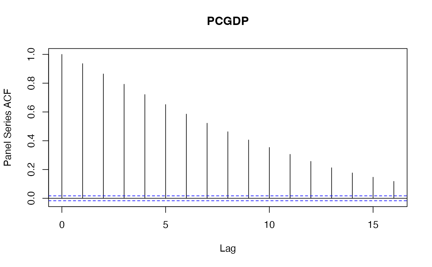
psacf(wlddev$PCGDP, wlddev$country, wlddev$year)                # ACF of GDP per Capita

psacf(wlddev, PCGDP ~ country, ~year)                           # Same using data.frame method

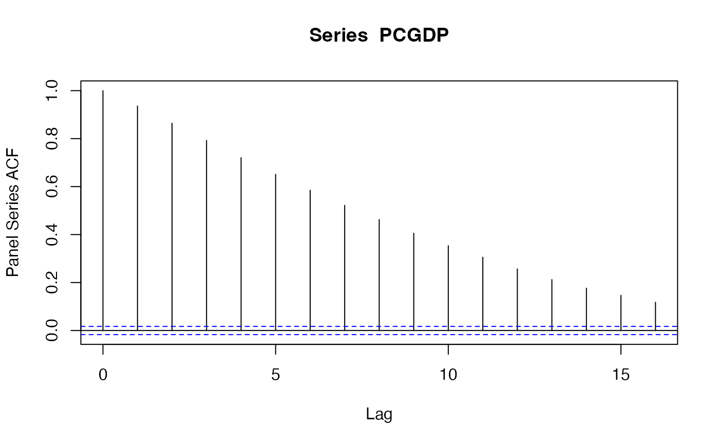
psacf(wlddev$PCGDP, wlddev$country)                             # The Data is sorted, can omit t

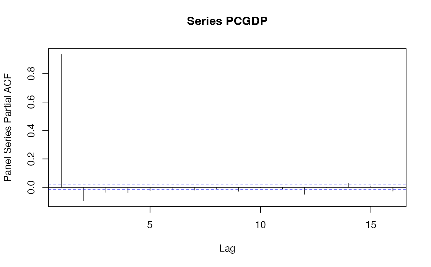
pspacf(wlddev$PCGDP, wlddev$country)                            # Partial ACF

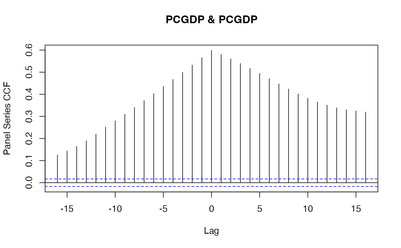
psccf(wlddev$PCGDP, wlddev$LIFEEX, wlddev$country)              # CCF with Life-Expectancy at Birth


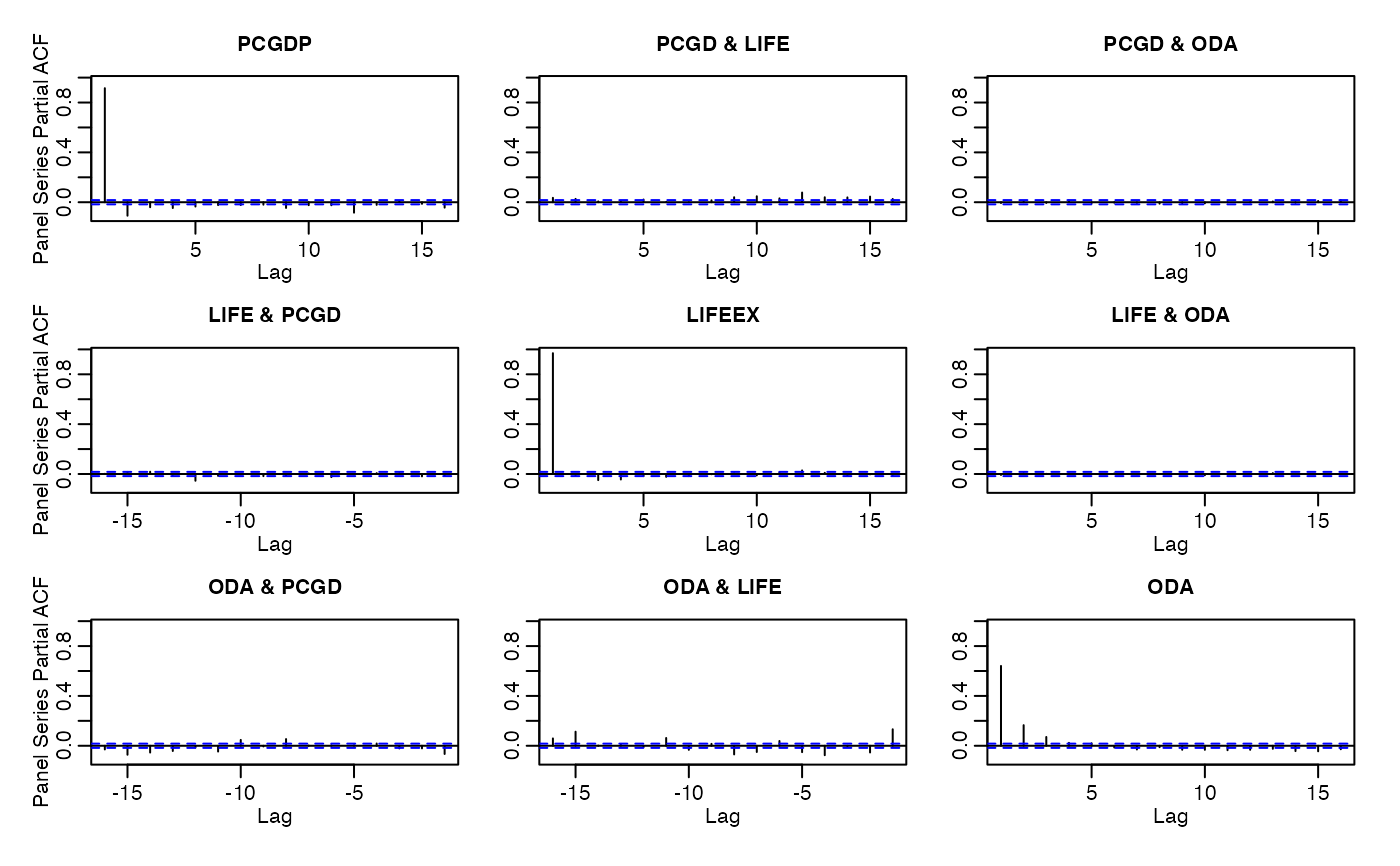
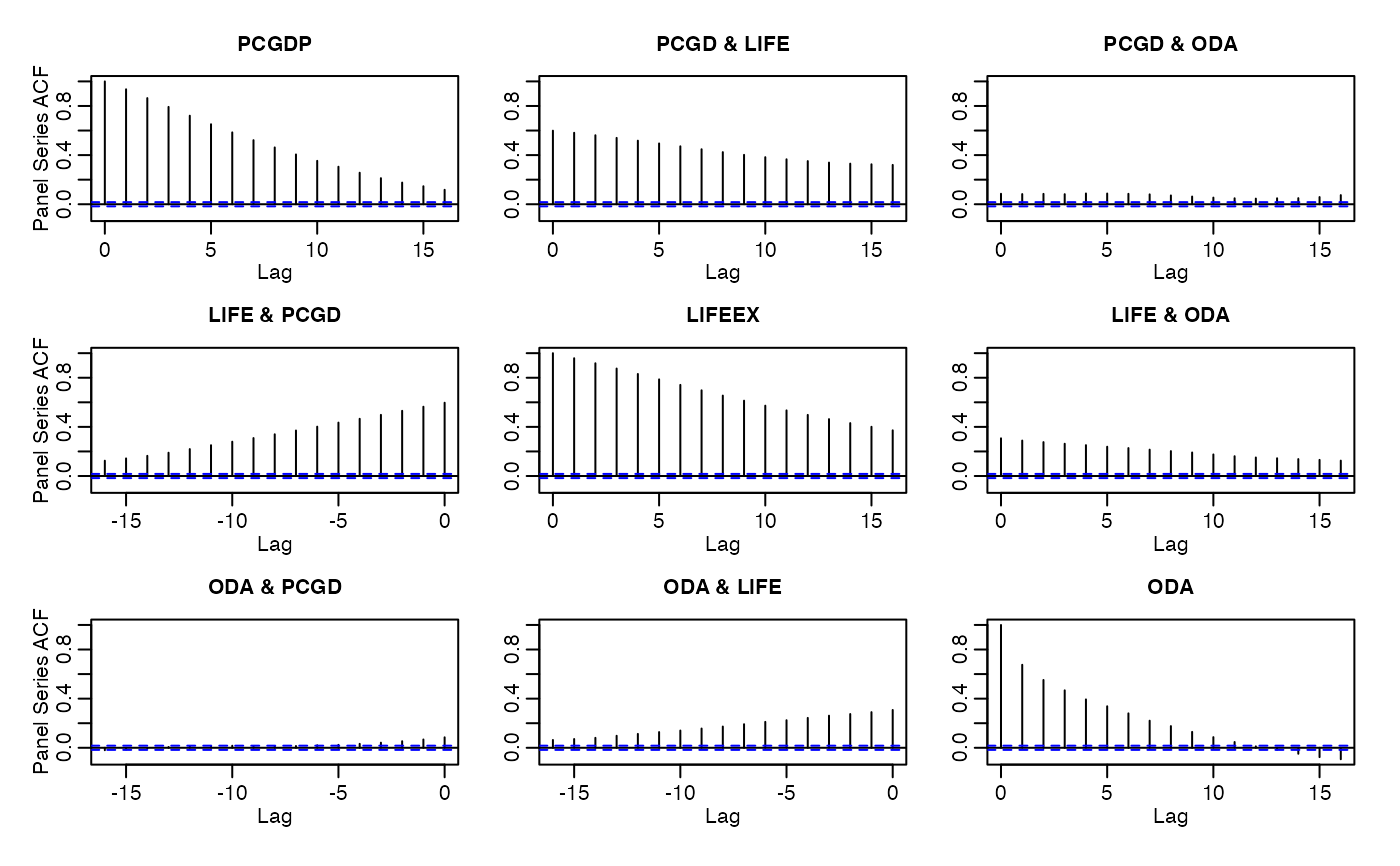
psacf(wlddev, PCGDP + LIFEEX + ODA ~ country, ~year)            # ACF and CCF of GDP, LIFEEX and ODA
psacf(wlddev, ~ country, ~year, c(9:10,12))                     # Same, using cols argument

pspacf(wlddev, ~ country, ~year, c(9:10,12))                    # Partial ACF


## Using indexed data:
wldi <- findex_by(wlddev, iso3c, year)  # Creating a indexed frame
PCGDP <- wldi$PCGDP                     # Indexed Series of GDP per Capita
LIFEEX <- wldi$LIFEEX                   # Indexed Series of Life Expectancy
psacf(PCGDP)                            # Same as above, more parsimonious

pspacf(PCGDP)

psccf(PCGDP, LIFEEX)

psacf(wldi[c(9:10,12)])

pspacf(wldi[c(9:10,12)])