Fast Indexed Time Series and Panels
indexing.RdA fast and flexible indexed time series and panel data class that inherits from plm's 'pseries' and 'pdata.frame', but is more rigorous, natively handles irregularity, can be superimposed on any data.frame/list, matrix or vector, and supports ad-hoc computations inside data masking functions and model formulas.
Usage
## Create an 'indexed_frame' containing 'indexed_series'
findex_by(.X, ..., single = "auto", interact.ids = TRUE)
iby(.X, ..., single = "auto", interact.ids = TRUE)  # Shorthand

## Retrieve the index ('index_df') from an 'indexed_frame' or 'indexed_series'
findex(x)
ix(x)     # Shorthand

## Remove index from 'indexed_frame' or 'indexed_series' (i.e. get .X back)
unindex(x)

## Reindex 'indexed_frame' or 'indexed_series' (or index vectors / matrices)
reindex(x, index = findex(x), single = "auto")

## Check if 'indexed_frame', 'indexed_series', index or time vector is irregular
is_irregular(x, any_id = TRUE)

## Convert 'indexed_frame'/'indexed_series' to normal 'pdata.frame'/'pseries'
to_plm(x, row.names = FALSE)

# Subsetting & replacement methods: [(<-) methods call NextMethod().
# Also methods for fsubset, funique and roworder(v), na_omit (internal).

# S3 method for class 'indexed_series'
x[i, ..., drop.index.levels = "id"]

# S3 method for class 'indexed_frame'
x[i, ..., drop.index.levels = "id"]

# S3 method for class 'indexed_frame'
x[i, j] <- value

# S3 method for class 'indexed_frame'
x$name

# S3 method for class 'indexed_frame'
x$name <- value

# S3 method for class 'indexed_frame'
x[[i, ...]]

# S3 method for class 'indexed_frame'
x[[i]] <- value

# Index subsetting and printing: optimized using ss()

# S3 method for class 'index_df'
x[i, j, drop = FALSE, drop.index.levels = "id"]

# S3 method for class 'index_df'
print(x, topn = 5, ...)
Arguments
- .X
a data frame or list-like object of equal-length columns.
- x
an 'indexed_frame' or 'indexed_series'.
findexalso works with 'pseries' and 'pdata.frame's created with plm. Foris_irregularxcan also be an index (inherits 'pindex') or a vector representing time.- ...
for
findex_by: variables identifying the individual (id) and/or time dimensions of the data. Passed either as unquoted comma-separated column names or (tagged) expressions involving columns, or as a vector of column names, indices, a logical vector or a selector function. The time variable must enter last. See Examples. Otherwise: further arguments passed toNextMethod().- single
character. If only one indexing variable is supplied, this can be declared as
"id"or"time"variable."auto"chooses"id"if the variable hasanyDuplicatedvalues.- interact.ids
logical. If
n > 2indexing variables are passed,TRUEcallsfinteractionon the firstn-1of them (n'th variable must be time).FALSEkeeps all variables in the index. The latter slows down computations of lags / differences etc. because ad-hoc interactions need to be computed, but gives more flexibility for scaling / centering / summarising over different data dimensions.- index
and index (inherits 'pindex'), or an atomic vector or list of factors matching the data dimensions. Atomic vectors or lists with 1 factor will must be declared, see
single. Atomic vectors will additionally be grouped / turned into time-factors. See Details.- drop.index.levels
character. Subset methods also subset the index (= a data.frame of factors), and this argument regulates which factor levels should be dropped: either
"all","id","time"or"none". The default"id"only drops levels from id's."all"or"time"should be used with caution because time-factors may contain levels for missing time periods (gaps in irregular sequences, or periods within a sequence removed through subsetting), and dropping those levels would create a variable that is ordinal but no longer represents time. The benefit of dropping levels is that it can speed-up subsequent computations by reducing the size of intermediate vectors created in C++.- any_id
logical. For panel series:
FALSEreturns the irregularity check performed for each id,TRUEcallsanyon those checks.- row.names
logical.
TRUEcreates descriptive row-names (or names for pseries) as inplm. This can be expensive and is usually not required forplmmodels to work.- topn
integer. The number of first and last rows to print.
- i, j, name, drop, value
Arguments passed to
NextMethod, or as in the data.frame methods. Note that for index subsetting to work,ineeds to be integer or logical (or an expression evaluation to integer or logical ifxis a data.table).
Details
The 'indexed_frame', 'indexed_series' and 'index_df' classes inherit plm's 'pdata.frame', 'pseries' and 'pindex' classes, respectively. They add, improve, and, in some cases, remove functionality offered by plm, with the aim of striking an optimal balance of flexibility and performance. The inheritance means that all 'pseries' and 'pdata.frame' methods in collapse, and also some methods in plm, apply to them.
The use of these classes does not require plm, but as a basic background: A 'pdata.frame' is a data.frame with an index attribute: a data.frame of 2 factors identifying the individual and time-dimension of the data. When pulling a variable out of the pdata.frame using a method like $.pdata.frame or [[.pdata.frame, a 'pseries' is created by transferring the index attribute to the vector. Methods defined for functions like lag / flag etc. use the index for correct computations on this panel data, also inside plm's estimation commands.
Main Features and Enhancements
The 'indexed_frame' and 'indexed_series' classes extend and enhance 'pdata.frame' and 'pseries' in a number of critical dimensions. Most notably they:
Support both time series and panel data, by allowing indexation of data with one, two or more variables.
Are class-agnostic: any data.frame/list (such as data.table, tibble, tsibble, sf etc.) can become an 'indexed_frame' and continue to function as usual for most use cases. Similarly, any vector or matrix (such as ts, mts, xts) can become an 'indexed_series'. This also allows for transient workflows e.g.
some_df |> findex_by(...) |> 'do something using collapse functions' |> unindex() |> 'continue working with some_df'.Have a comprehensive and efficient set of methods for subsetting and manipulation, including methods for
fsubset,funique,roworder(v)(internal) andna_omit(internal,na.omitalso works but is slower). It is also possible to group indexed data withfgroup_byfor transformations e.g. usingfmutate, but aggregation requiresunindex()ing.Natively handle irregularity: time objects (such as 'Date', 'POSIXct' etc.) are passed to
timeid, which efficiently determines the temporal structure by finding the greatest common divisor (GCD), and creates a time-factor with levels corresponding to a complete time-sequence. Plain numeric vectors are assumed to represent unit time steps (GDC = 1) and coerced to integer (but can also be passed throughtimeidif non-unitary). Character time variables are converted to factor. Using this time-factor in the index, collapse's functions efficiently perform correct computations on irregular sequences and panels without the need to 'expand' the data / fill gaps.is_irregularcan be used to check for irregularity in the entire sequence / panel or separately for each individual in panel data.Support computations inside data-masking functions and formulas, by virtue of "deep indexation": Each variable inside an 'indexed_frame' is an 'indexed_series' which contains in its 'index_df' attribute an external pointer to the 'index_df' attribute of the frame. Functions operating on 'indexed_series' stored inside the frame (such as
with(data, flag(column))) can fetch the index from this pointer. This allows worry-free application inside arbitrary data masking environments (with,%$%,attach, etc..) and estimation commands (glm,feols,lmrobetc..) without duplication of the index in memory. A limitation is that external pointers are only valid during the present R session, thus when saving an 'indexed_frame' and loading it again, you need to calldata = reindex(data)before computing on it.
Indexed series also have simple Math and Ops methods, which apply the operation to the unindexed series and shallow copy the attributes of the original object to the result, unless the result it is a logical vector (from operations like !, == etc.). For Ops methods, if the LHS object is an 'indexed_series' its attributes are taken, otherwise the attributes of the RHS object are taken.
Limits to plm Compatibility
In contrast to 'pseries' and 'pdata.frame's, 'indexed_series' and 'indexed_frames' do not have descriptive "names" or "row.names" attributes attached to them, mainly for efficiency reasons.
Furthermore, the index is stored in an attribute named 'index_df' (same as the class name), not 'index' as in plm, mainly to make these classes work with data.table, tsibble and xts, which also utilize 'index' attributes. This for the most part poses no problem to plm compatibility because plm source code fetches the index using attr(x, "index"), and attr by default performs partial matching.
A much greater obstacle in working with plm is that some internal plm code is hinged on there being no [.pseries method, and the existence of [.indexed_series limits the use of these classes in most plm estimation commands. Therefore the to_plm function is provided to efficiently coerce the classes to ordinary plm objects before estimation. See Examples.
Overall these classes don't really benefit plm, especially given that collapse's plm methods also support native plm objects.
Performance Considerations
When indexing long time-series or panels with a single variable, setting single = "id" or "time" avoids a potentially expensive call to anyDuplicated. Note also that when panel-data are regular and sorted, omitting the time variable in the index can bring >= 2x performance improvements in operations like lagging and differencing (alternatively use shift = "row" argument to flag, fdiff etc.) .
When dealing with long Date or POSIXct time sequences, it may also be that the internal processing by timeid is slow simply because calling strftime on these sequences to create factor levels is slow. In this case you may choose to generate an index factor with integer levels by passing timeid(t) to findex_by or reindex (which by default generates a 'qG' object which is internally converted to factor using as_factor_qG. The lazy evaluation of expressions like as.character(seq_len(nlev)) in modern R makes this extremely efficient).
With multiple id variables e.g. findex_by(data, id1, id2, id3, time), the default call to finteraction() can be expensive because of pasting the levels together. In this case, users may gain performance by invoking group(), e.g. findex_by(data, ids = group(id1, id2, id3), time). This will generate a factor with integer levels instead.
Print Method
The print methods for 'indexed_frame' and 'indexed_series' first call print(unindex(x), ...), followed by the index variables with the number of categories (index factor levels) in square brackets. If the time factor contains unused levels (= irregularity in the sequence), the square brackets indicate the number of used levels (periods), followed by the total number of levels (periods in the sequence) in parentheses.
Examples
oldopts <- options(max.print = 70)
# Indexing panel data ----------------------------------------------------------
wldi <- findex_by(wlddev, iso3c, year)
wldi
#> country iso3c date year decade region income OECD PCGDP
#> 1 Afghanistan AFG 1961-01-01 1960 1960 South Asia Low income FALSE NA
#> 2 Afghanistan AFG 1962-01-01 1961 1960 South Asia Low income FALSE NA
#> 3 Afghanistan AFG 1963-01-01 1962 1960 South Asia Low income FALSE NA
#> 4 Afghanistan AFG 1964-01-01 1963 1960 South Asia Low income FALSE NA
#> 5 Afghanistan AFG 1965-01-01 1964 1960 South Asia Low income FALSE NA
#> LIFEEX GINI ODA POP
#> 1 32.446 NA 116769997 8996973
#> 2 32.962 NA 232080002 9169410
#> 3 33.471 NA 112839996 9351441
#> 4 33.971 NA 237720001 9543205
#> 5 34.463 NA 295920013 9744781
#> [ reached 'max' / getOption("max.print") -- omitted 13171 rows ]
#>
#> Indexed by: iso3c [216] | year [61]
wldi[1:100,1] # Works like a data frame
#> [1] "Afghanistan" "Afghanistan" "Afghanistan" "Afghanistan" "Afghanistan"
#> [6] "Afghanistan" "Afghanistan" "Afghanistan" "Afghanistan" "Afghanistan"
#> [11] "Afghanistan" "Afghanistan" "Afghanistan" "Afghanistan" "Afghanistan"
#> [16] "Afghanistan" "Afghanistan" "Afghanistan" "Afghanistan" "Afghanistan"
#> [21] "Afghanistan" "Afghanistan" "Afghanistan" "Afghanistan" "Afghanistan"
#> [26] "Afghanistan" "Afghanistan" "Afghanistan" "Afghanistan" "Afghanistan"
#> [31] "Afghanistan" "Afghanistan" "Afghanistan" "Afghanistan" "Afghanistan"
#> [36] "Afghanistan" "Afghanistan" "Afghanistan" "Afghanistan" "Afghanistan"
#> [41] "Afghanistan" "Afghanistan" "Afghanistan" "Afghanistan" "Afghanistan"
#> [46] "Afghanistan" "Afghanistan" "Afghanistan" "Afghanistan" "Afghanistan"
#> [51] "Afghanistan" "Afghanistan" "Afghanistan" "Afghanistan" "Afghanistan"
#> [56] "Afghanistan" "Afghanistan" "Afghanistan" "Afghanistan" "Afghanistan"
#> [61] "Afghanistan" "Albania" "Albania" "Albania" "Albania"
#> [66] "Albania" "Albania" "Albania" "Albania" "Albania"
#> [ reached 'max' / getOption("max.print") -- omitted 30 entries ]
#>
#> Indexed by: iso3c [2] | year [61]
POP <- wldi$POP # indexed_series
qsu(POP) # Summary statistics
#> N/T Mean SD Min Max
#> Overall 12919 24'245971.6 102'120674 2833 1.39771500e+09
#> Between 216 24'178573 98'616506.7 8343.3333 1.08786967e+09
#> Within 59.8102 24'245971.6 26'803077.4 -405'793067 510'077008
G(POP) # Population growth
#> [1] NA 1.9166113 1.9851986 2.0506358 2.1122464 2.1707928
#> [7] 2.1947467 2.2122224 2.2801797 2.4133823 2.5690449 2.7010262
#> [13] 2.7517016 2.6947859 2.5104297 2.2251761 2.0011805 1.7632030
#> [19] 1.2898645 0.5236261 -0.4067167 -1.3838794 -2.1952033 -2.6764778
#> [25] -2.6594766 -2.1802494 -1.6922892 -1.1217024 0.1160839 2.1593380
#> [31] 4.5786219 7.1437882 8.9219301 9.1888632 7.9607739 6.0608254
#> [37] 4.1013421 2.6716031 1.9664025 2.1941643 3.0197497 3.9799657
#> [43] 4.5993546 4.7790451 4.4162776 3.7513845 3.0356420 2.5251987
#> [49] 2.2941982 2.4259805 2.7846424 3.1930437 3.4663103 3.5563673
#> [55] 3.4125163 3.1249152 2.8172726 2.5810946 2.4134239 2.3387468
#> [61] NA NA 3.1700646 3.1039282 2.9978046 2.9225795
#> [67] 2.7922950 2.6695753 2.6650851 2.8832956
#> [ reached 'max' / getOption("max.print") -- omitted 13106 entries ]
#> attr(,"label")
#> [1] "Population, total"
#>
#> Indexed by: iso3c [216] | year [61]
STD(G(POP, c(1, 10))) # Within-standardized 1 and 10-year growth rates
#> G1 L10G1
#> [1,] NA NA
#> [2,] -2.404379e-01 NA
#> [3,] -2.122758e-01 NA
#> [4,] -1.854071e-01 NA
#> [5,] -1.601097e-01 NA
#> [6,] -1.360704e-01 NA
#> [7,] -1.262349e-01 NA
#> [8,] -1.190593e-01 NA
#> [9,] -9.115593e-02 NA
#> [10,] -3.646264e-02 NA
#> [11,] 2.745275e-02 -2.502986e-01
#> [12,] 8.164455e-02 -2.072055e-01
#> [13,] 1.024520e-01 -1.648010e-01
#> [14,] 7.908227e-02 -1.289204e-01
#> [15,] 3.385202e-03 -1.066142e-01
#> [16,] -1.137405e-01 -1.035575e-01
#> [17,] -2.057136e-01 -1.144404e-01
#> [18,] -3.034277e-01 -1.396334e-01
#> [19,] -4.977815e-01 -1.949160e-01
#> [20,] -8.124006e-01 -2.992510e-01
#> [21,] -1.194401e+00 -4.602688e-01
#> [22,] -1.595626e+00 -6.746138e-01
#> [23,] -1.928758e+00 -9.237424e-01
#> [24,] -2.126370e+00 -1.181362e+00
#> [25,] -2.119389e+00 -1.416777e+00
#> [26,] -1.922618e+00 -1.607795e+00
#> [27,] -1.722260e+00 -1.761378e+00
#> [28,] -1.487976e+00 -1.877266e+00
#> [29,] -9.797383e-01 -1.923294e+00
#> [30,] -1.407738e-01 -1.859412e+00
#> [31,] 8.525893e-01 -1.659693e+00
#> [32,] 1.905852e+00 -1.297409e+00
#> [33,] 2.635961e+00 -7.800175e-01
#> [34,] 2.745564e+00 -1.619956e-01
#> [35,] 2.241308e+00 4.585063e-01
#> [ reached 'max' / getOption("max.print") -- omitted 13141 rows ]
#> attr(,"label")
#> [1] "Population, total"
#> attr(,"class")
#> [1] "numeric" "matrix"
#>
#> Indexed by: iso3c [216] | year [61]
psmat(POP) # Panel-Series Matrix
#> 1960 1961 1962 1963 1964 1965 1966 1967
#> ABW 5.42e+04 5.54e+04 5.62e+04 5.67e+04 5.70e+04 5.74e+04 5.77e+04 5.81e+04
#> 1968 1969 1970 1971 1972 1973 1974 1975
#> ABW 5.84e+04 5.87e+04 5.91e+04 5.94e+04 5.98e+04 6.02e+04 6.05e+04 6.07e+04
#> 1976 1977 1978 1979 1980 1981 1982 1983
#> ABW 6.06e+04 6.04e+04 6.01e+04 6.00e+04 6.01e+04 6.06e+04 6.13e+04 6.22e+04
#> 1984 1985 1986 1987 1988 1989 1990 1991
#> ABW 6.28e+04 6.30e+04 6.26e+04 6.18e+04 6.11e+04 6.10e+04 6.21e+04 6.46e+04
#> 1992 1993 1994 1995 1996 1997 1998 1999
#> ABW 6.82e+04 7.25e+04 7.67e+04 8.03e+04 8.32e+04 8.55e+04 8.73e+04 8.90e+04
#> 2000 2001 2002 2003 2004 2005 2006 2007
#> ABW 9.09e+04 9.29e+04 9.50e+04 9.70e+04 9.87e+04 1.00e+05 1.01e+05 1.01e+05
#> 2008 2009 2010 2011 2012 2013 2014 2015
#> ABW 1.01e+05 1.01e+05 1.02e+05 1.02e+05 1.03e+05 1.03e+05 1.04e+05 1.04e+05
#> 2016 2017 2018 2019 2020
#> ABW 1.05e+05 1.05e+05 1.06e+05 1.06e+05 NA
#> [ reached 'max' / getOption("max.print") -- omitted 215 rows ]
plot(psmat(log10(POP)))
 POP[30:5000] # Subsetting indexed_series
#> [1] 11868877 12412308 13299017 14485546 15816603 17075727 18110657 18853437
#> [9] 19357126 19737765 20170844 20779953 21606988 22600770 23680871 24726684
#> [17] 25654277 26433049 27100536 27722276 28394813 29185507 30117413 31161376
#> [25] 32269589 33370794 34413603 35383128 36296400 37172386 38041754 NA
#> [33] 1608800 1659800 1711319 1762621 1814135 1864791 1914573 1965598
#> [41] 2022272 2081695 2135479 2187853 2243126 2296752 2350124 2404831
#> [49] 2458526 2513546 2566266 2617832 2671997 2726056 2784278 2843960
#> [57] 2904429 2964762 3022635 3083605 3142336 3227943 3286542 3266790
#> [65] 3247039 3227287 3207536 3187784 3168033 3148281
#> [ reached 'max' / getOption("max.print") -- omitted 4901 entries ]
#>
#> Indexed by: iso3c [82] | year [61]
Dlog(POP[30:5000]) # Log-difference of subset
#> [1] NA 0.044768965 0.069001562 0.085461202 0.087908886
#> [6] 0.076597770 0.058842568 0.040194682 0.026365389 0.019473185
#> [11] 0.021704390 0.029750528 0.039028057 0.044967196 0.046683615
#> [16] 0.043215393 0.036827318 0.029904781 0.024938423 0.022682771
#> [21] 0.023970210 0.027465763 0.031431259 0.034075870 0.034945890
#> [26] 0.033555817 0.030770836 0.027783174 0.025483466 0.023847611
#> [31] 0.023118172 NA NA 0.031208554 0.030567305
#> [36] 0.029537488 0.028806864 0.027540212 0.026345639 0.026301903
#> [41] 0.028425107 0.028960834 0.025508512 0.024229720 0.024949731
#> [46] 0.023625522 0.022972142 0.023011538 0.022082353 0.022132522
#> [51] 0.020757419 0.019894570 0.020479639 0.020029743 0.021132718
#> [56] 0.021208853 0.021039366 0.020559946 0.019332208 0.019970400
#> [61] 0.018867105 0.026878620 0.017990856 -0.006028097 -0.006064347
#> [66] -0.006101658 -0.006138805 -0.006177037 -0.006215114 -0.006254301
#> [ reached 'max' / getOption("max.print") -- omitted 4901 entries ]
#>
#> Indexed by: iso3c [82] | year [61]
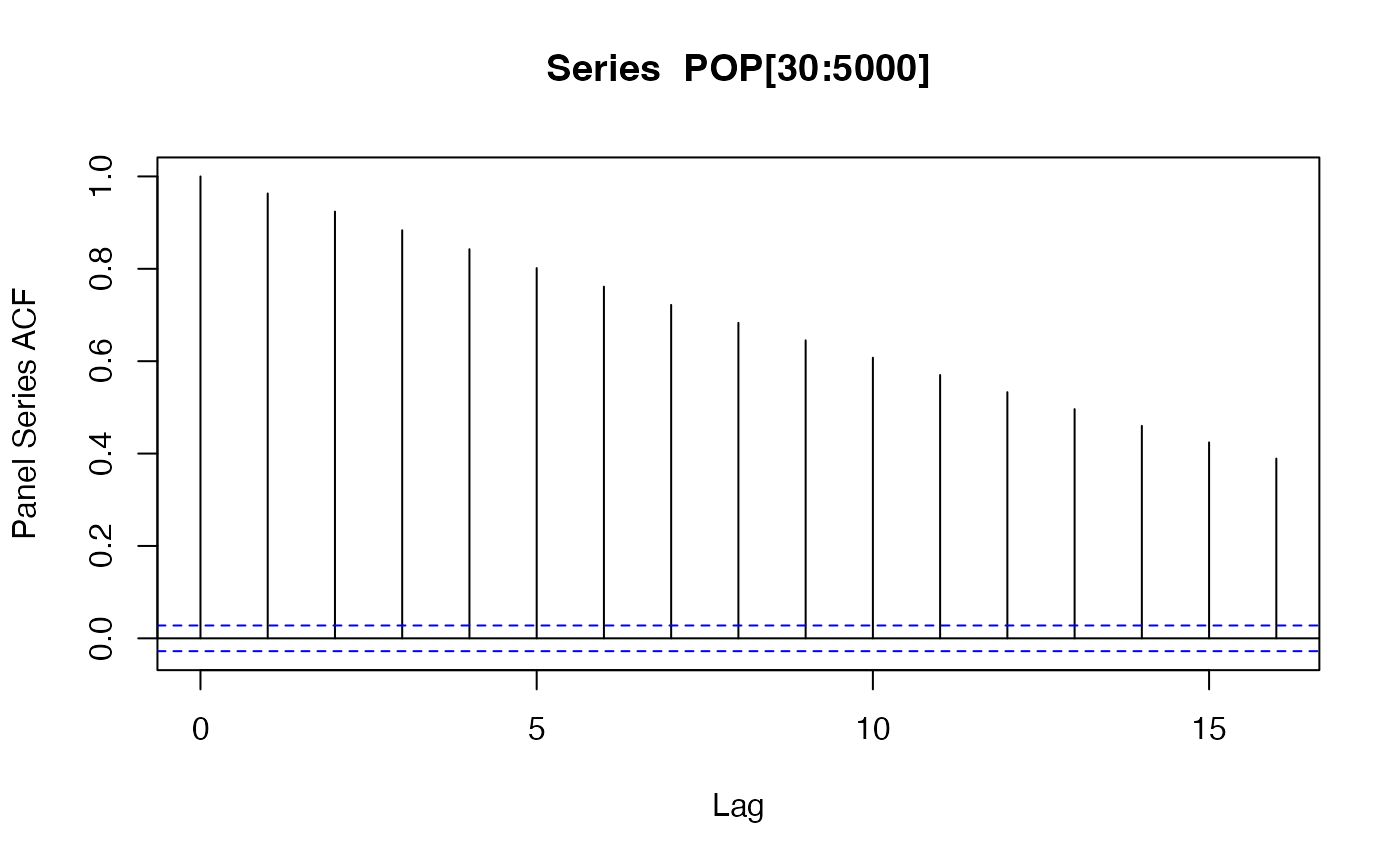
psacf(identity(POP[30:5000])) # ACF of subset
POP[30:5000] # Subsetting indexed_series
#> [1] 11868877 12412308 13299017 14485546 15816603 17075727 18110657 18853437
#> [9] 19357126 19737765 20170844 20779953 21606988 22600770 23680871 24726684
#> [17] 25654277 26433049 27100536 27722276 28394813 29185507 30117413 31161376
#> [25] 32269589 33370794 34413603 35383128 36296400 37172386 38041754 NA
#> [33] 1608800 1659800 1711319 1762621 1814135 1864791 1914573 1965598
#> [41] 2022272 2081695 2135479 2187853 2243126 2296752 2350124 2404831
#> [49] 2458526 2513546 2566266 2617832 2671997 2726056 2784278 2843960
#> [57] 2904429 2964762 3022635 3083605 3142336 3227943 3286542 3266790
#> [65] 3247039 3227287 3207536 3187784 3168033 3148281
#> [ reached 'max' / getOption("max.print") -- omitted 4901 entries ]
#>
#> Indexed by: iso3c [82] | year [61]
Dlog(POP[30:5000]) # Log-difference of subset
#> [1] NA 0.044768965 0.069001562 0.085461202 0.087908886
#> [6] 0.076597770 0.058842568 0.040194682 0.026365389 0.019473185
#> [11] 0.021704390 0.029750528 0.039028057 0.044967196 0.046683615
#> [16] 0.043215393 0.036827318 0.029904781 0.024938423 0.022682771
#> [21] 0.023970210 0.027465763 0.031431259 0.034075870 0.034945890
#> [26] 0.033555817 0.030770836 0.027783174 0.025483466 0.023847611
#> [31] 0.023118172 NA NA 0.031208554 0.030567305
#> [36] 0.029537488 0.028806864 0.027540212 0.026345639 0.026301903
#> [41] 0.028425107 0.028960834 0.025508512 0.024229720 0.024949731
#> [46] 0.023625522 0.022972142 0.023011538 0.022082353 0.022132522
#> [51] 0.020757419 0.019894570 0.020479639 0.020029743 0.021132718
#> [56] 0.021208853 0.021039366 0.020559946 0.019332208 0.019970400
#> [61] 0.018867105 0.026878620 0.017990856 -0.006028097 -0.006064347
#> [66] -0.006101658 -0.006138805 -0.006177037 -0.006215114 -0.006254301
#> [ reached 'max' / getOption("max.print") -- omitted 4901 entries ]
#>
#> Indexed by: iso3c [82] | year [61]
psacf(identity(POP[30:5000])) # ACF of subset
 L(Dlog(POP[30:5000], c(1, 10)), -1:1) # Multiple computations on subset
#> F1.Dlog1 Dlog1 L1.Dlog1 F1.L10Dlog1 L10Dlog1
#> [1,] 4.476897e-02 NA NA NA NA
#> [2,] 6.900156e-02 4.476897e-02 NA NA NA
#> [3,] 8.546120e-02 6.900156e-02 4.476897e-02 NA NA
#> [4,] 8.790889e-02 8.546120e-02 6.900156e-02 NA NA
#> [5,] 7.659777e-02 8.790889e-02 8.546120e-02 NA NA
#> [6,] 5.884257e-02 7.659777e-02 8.790889e-02 NA NA
#> [7,] 4.019468e-02 5.884257e-02 7.659777e-02 NA NA
#> [8,] 2.636539e-02 4.019468e-02 5.884257e-02 NA NA
#> [9,] 1.947319e-02 2.636539e-02 4.019468e-02 NA NA
#> [10,] 2.170439e-02 1.947319e-02 2.636539e-02 0.5303185995 NA
#> [11,] 2.975053e-02 2.170439e-02 1.947319e-02 0.5153001629 0.5303185995
#> L1.L10Dlog1
#> [1,] NA
#> [2,] NA
#> [3,] NA
#> [4,] NA
#> [5,] NA
#> [6,] NA
#> [7,] NA
#> [8,] NA
#> [9,] NA
#> [10,] NA
#> [11,] NA
#> [ reached 'max' / getOption("max.print") -- omitted 4960 rows ]
#> attr(,"class")
#> [1] "numeric" "matrix"
#>
#> Indexed by: iso3c [82] | year [61]
# Fast Statistical Functions don't have dedicated methods
# Thus for aggregation we need to unindex beforehand ...
fmean(unindex(POP))
#> [1] 24245972
#> attr(,"label")
#> [1] "Population, total"
wldi |> unindex() |>
fgroup_by(iso3c) |> num_vars() |> fmean()
#> iso3c year decade PCGDP LIFEEX GINI ODA POP
#> 1 ABW 1990 1985.574 25413.8370 72.40653 NA 33245000 76268.63
#> 2 AFG 1990 1985.574 483.8351 49.19717 NA 1487548499 18362258.22
#> 3 AGO 1990 1985.574 2887.6879 46.75805 48.66667 267452068 13823228.03
#> 4 ALB 1990 1985.574 2819.2400 71.68027 31.41111 312928126 2708297.17
#> 5 AND 1990 1985.574 40083.0911 NA NA NA 51547.35
#> 6 ARE 1990 1985.574 64616.4864 69.37793 29.25000 13384222 3089064.62
#> 7 ARG 1990 1985.574 7907.8326 71.12565 45.92258 106930833 32301197.52
#> 8 ARM 1990 1985.574 2520.1808 70.67953 32.24500 282426894 2912376.95
#> [ reached 'max' / getOption("max.print") -- omitted 208 rows ]
library(magrittr)
# ... or unindex after taking group identifiers from the index
fmean(unindex(fgrowth(POP)), ix(POP)$iso3c)
#> ABW AFG AGO ALB AND ARE
#> 1.15986116 2.50218519 3.04019111 0.98728941 3.03828499 8.33912222
#> ARG ARM ASM ATG AUS AUT
#> 1.34100846 0.78894579 1.74127860 0.99964449 1.54424580 0.39301937
#> AZE BDI BEL BEN BFA BGD
#> 1.61742943 2.43172184 0.38832202 2.71473569 2.46698310 2.09594336
#> BGR BHR BHS BIH BLR BLZ
#> -0.20095889 4.01156764 2.17972600 0.04870005 0.23697183 2.48033866
#> BMU BOL BRA BRB BRN BTN
#> 0.62656641 1.96310764 1.83756339 0.36894714 2.87598784 2.10961311
#> BWA CAF CAN CHE CHI CHL
#> 2.61689824 1.97141241 1.26547829 0.81130910 0.77252949 1.44461721
#> CHN CIV CMR COD COG COL
#> 1.26475057 3.43990856 2.76520875 2.99210471 2.86194380 1.95730439
#> COM CPV CRI CUB CUW CYM
#> 2.56471792 1.71779560 2.28825488 0.78844375 0.40380104 3.65940831
#> CYP CZE DEU DJI DMA DNK
#> 1.26066375 0.17964024 0.22511110 4.28964392 0.30770228 0.40573747
#> DOM DZA ECU EGY ERI ESP
#> 2.02552207 2.33239690 2.30053844 2.27489144 2.30900292 0.74430651
#> EST ETH FIN FJI FRA FRO
#> 0.15848536 2.78733512 0.37433864 1.39760426 0.61832292 0.58122004
#> FSM GAB GBR GEO
#> 1.61438473 2.51981406 0.41364183 0.04208078
#> [ reached 'max' / getOption("max.print") -- omitted 146 entries ]
#> attr(,"label")
#> [1] "Population, total"
wldi |> num_vars() %>%
fgroup_by(iso3c = ix(.)$iso3c) |>
unindex() |> fmean()
#> iso3c year decade PCGDP LIFEEX GINI ODA POP
#> 1 ABW 1990 1985.574 25413.8370 72.40653 NA 33245000 76268.63
#> 2 AFG 1990 1985.574 483.8351 49.19717 NA 1487548499 18362258.22
#> 3 AGO 1990 1985.574 2887.6879 46.75805 48.66667 267452068 13823228.03
#> 4 ALB 1990 1985.574 2819.2400 71.68027 31.41111 312928126 2708297.17
#> 5 AND 1990 1985.574 40083.0911 NA NA NA 51547.35
#> 6 ARE 1990 1985.574 64616.4864 69.37793 29.25000 13384222 3089064.62
#> 7 ARG 1990 1985.574 7907.8326 71.12565 45.92258 106930833 32301197.52
#> 8 ARM 1990 1985.574 2520.1808 70.67953 32.24500 282426894 2912376.95
#> [ reached 'max' / getOption("max.print") -- omitted 208 rows ]
# With matrix methods it is easier as most attributes are dropped upon aggregation.
G(POP, c(1, 10)) %>% fmean(ix(.)$iso3c)
#> G1 L10G1
#> ABW 1.15986116 13.5405797
#> AFG 2.50218519 29.7453631
#> AGO 3.04019111 37.2423846
#> ALB 0.98728941 10.4611010
#> AND 3.03828499 36.8630696
#> ARE 8.33912222 145.2957118
#> ARG 1.34100846 14.3289740
#> ARM 0.78894579 7.1746628
#> ASM 1.74127860 20.2992819
#> ATG 0.99964449 10.0195522
#> AUS 1.54424580 16.0434792
#> AUT 0.39301937 3.5211125
#> AZE 1.61742943 16.4526447
#> BDI 2.43172184 26.7915415
#> BEL 0.38832202 3.6354631
#> BEN 2.71473569 31.9252634
#> BFA 2.46698310 28.3385127
#> BGD 2.09594336 23.3556445
#> BGR -0.20095889 -2.3160917
#> BHR 4.01156764 50.7327853
#> BHS 2.17972600 22.6999691
#> BIH 0.04870005 0.5070281
#> BLR 0.23697183 2.1725510
#> BLZ 2.48033866 27.8347280
#> BMU 0.62656641 5.7036637
#> BOL 1.96310764 21.9315509
#> BRA 1.83756339 20.1289837
#> BRB 0.36894714 3.9565564
#> BRN 2.87598784 33.4451942
#> BTN 2.10961311 23.9024113
#> BWA 2.61689824 31.1856395
#> CAF 1.97141241 22.7889510
#> CAN 1.26547829 12.8834454
#> CHE 0.81130910 7.3670756
#> CHI 0.77252949 7.6461689
#> [ reached 'max' / getOption("max.print") -- omitted 181 rows ]
# Example of index with multiple ids
GGDC10S |> findex_by(Variable, Country, Year) |> head() # default is interact.ids = TRUE
#> Country Regioncode Region Variable Year AGR MIN MAN PU CON WRT
#> 1 BWA SSA Sub-saharan Africa VA 1960 NA NA NA NA NA NA
#> 2 BWA SSA Sub-saharan Africa VA 1961 NA NA NA NA NA NA
#> 3 BWA SSA Sub-saharan Africa VA 1962 NA NA NA NA NA NA
#> 4 BWA SSA Sub-saharan Africa VA 1963 NA NA NA NA NA NA
#> TRA FIRE GOV OTH SUM
#> 1 NA NA NA NA NA
#> 2 NA NA NA NA NA
#> 3 NA NA NA NA NA
#> 4 NA NA NA NA NA
#> [ reached 'max' / getOption("max.print") -- omitted 2 rows ]
#>
#> Indexed by: Variable.Country [1] | Year [6 (67)]
GGDCi <- GGDC10S |> findex_by(Variable, Country, Year, interact.ids = FALSE)
head(GGDCi)
#> Country Regioncode Region Variable Year AGR MIN MAN PU CON WRT
#> 1 BWA SSA Sub-saharan Africa VA 1960 NA NA NA NA NA NA
#> 2 BWA SSA Sub-saharan Africa VA 1961 NA NA NA NA NA NA
#> 3 BWA SSA Sub-saharan Africa VA 1962 NA NA NA NA NA NA
#> 4 BWA SSA Sub-saharan Africa VA 1963 NA NA NA NA NA NA
#> TRA FIRE GOV OTH SUM
#> 1 NA NA NA NA NA
#> 2 NA NA NA NA NA
#> 3 NA NA NA NA NA
#> 4 NA NA NA NA NA
#> [ reached 'max' / getOption("max.print") -- omitted 2 rows ]
#>
#> Indexed by: Variable [1] Country [1] | Year [6 (67)]
findex(GGDCi)
#> Variable Country Year
#> 1 VA BWA 1960
#> 2 VA BWA 1961
#> 3 VA BWA 1962
#> 4 VA BWA 1963
#> 5 VA BWA 1964
#> ---
#> 5023 EMP EGY 2008
#> 5024 EMP EGY 2009
#> 5025 EMP EGY 2010
#> 5026 EMP EGY 2011
#> 5027 EMP EGY 2012
#>
#> Variable [2] Country [43] | Year [67]
# The benefit is increased flexibility for summary statistics and data transformation
qsu(GGDCi, effect = "Country")
#> , , Country
#>
#> N/T Mean SD Min Max
#> Overall 5027 - - - -
#> Between 43 - - - -
#> Within 116.907 - - - -
#>
#> , , Regioncode
#>
#> N/T Mean SD Min Max
#> Overall 5027 - - - -
#> Between 43 - - - -
#> Within 116.907 - - - -
#>
#> , , Region
#>
#> N/T Mean SD Min Max
#> Overall 5027 - - - -
#> Between 43 - - - -
#> Within 116.907 - - - -
#>
#> , , Variable
#>
#> N/T Mean SD Min Max
#> Overall 5027 - - - -
#> Between 43 - - - -
#> Within 116.907 - - - -
#>
#> , , Year
#>
#> N/T Mean SD Min Max
#> Overall 5027 1981.5801 17.5704 1947 2013
#> Between 43 1982.4236 5.0799 1978.7519 2011.5
#>
#> [ reached 'max' / getOption("max.print") -- omitted 11 slices ]
STD(GGDCi$SUM, effect = "Variable") # Standardizing by variable
#> [1] NA NA NA NA -0.1226776 -0.1226776
#> [7] -0.1226776 -0.1226776 -0.1226776 -0.1226776 -0.1226775 -0.1226775
#> [13] -0.1226774 -0.1226773 -0.1226772 -0.1226771 -0.1226769 -0.1226767
#> [19] -0.1226766 -0.1226762 -0.1226756 -0.1226753 -0.1226752 -0.1226744
#> [25] -0.1226738 -0.1226724 -0.1226704 -0.1226692 -0.1226661 -0.1226627
#> [31] -0.1226607 -0.1226582 -0.1226567 -0.1226550 -0.1226499 -0.1226448
#> [37] -0.1226376 -0.1226320 -0.1226275 -0.1226148 -0.1226044 -0.1225979
#> [43] -0.1225908 -0.1225861 -0.1225770 -0.1225543 -0.1225338 -0.1225158
#> [49] -0.1224963 -0.1225084 -0.1224488 NA NA NA
#> [55] NA NA -0.3807465 -0.3806958 -0.3806859 -0.3806942
#> [61] -0.3806630 -0.3805993 -0.3805239 -0.3804590 -0.3803244 -0.3802321
#> [67] -0.3801543 -0.3800409 -0.3799774 -0.3799017
#> [ reached 'max' / getOption("max.print") -- omitted 4957 entries ]
#> attr(,"label")
#> [1] "Summation of sector GDP"
#> attr(,"format.stata")
#> [1] "%10.0g"
#>
#> Indexed by: Variable [2] Country [43] | Year [67]
STD(GGDCi$SUM, effect = c("Variable", "Year")) # ... by variable and year
#> [1] NA NA NA NA -0.2041456 -0.2039970
#> [7] -0.2023122 -0.2041736 -0.2058182 -0.2068329 -0.1799561 -0.1784717
#> [13] -0.1794400 -0.1809847 -0.1852166 -0.1881118 -0.1915147 -0.1952319
#> [19] -0.2000250 -0.2086539 -0.2176069 -0.2246298 -0.2285386 -0.2384116
#> [25] -0.2442721 -0.2480965 -0.2533789 -0.2618757 -0.2684392 -0.2739245
#> [31] -0.2788689 -0.2831778 -0.2934982 -0.3006316 -0.3052873 -0.3081273
#> [37] -0.3074253 -0.3039395 -0.2818521 -0.2751017 -0.2694049 -0.2606845
#> [43] -0.2576762 -0.2567207 -0.2531264 -0.2434613 -0.2351500 -0.2288238
#> [49] -0.2182615 -0.2127535 -0.2090734 NA NA NA
#> [55] NA NA -0.4596772 -0.4497862 -0.4399738 -0.4363115
#> [61] -0.4331453 -0.4247106 -0.4027655 -0.4096142 -0.4114065 -0.4141980
#> [67] -0.4082425 -0.4024895 -0.4026850 -0.4047382
#> [ reached 'max' / getOption("max.print") -- omitted 4957 entries ]
#> attr(,"label")
#> [1] "Summation of sector GDP"
#> attr(,"format.stata")
#> [1] "%10.0g"
#>
#> Indexed by: Variable [2] Country [43] | Year [67]
# But time-based operations are a bit more expensive because of the necessary interactions
D(GGDCi$SUM)
#> [1] NA NA NA NA NA
#> [6] 1.8648058 3.7996670 -1.7515810 -0.2525958 10.0790095
#> [11] 15.2179271 12.1300779 31.7872318 37.4213552 35.1940244
#> [16] 36.8116252 85.0015379 44.7177833 52.5841475 158.9853717
#> [21] 198.2115288 103.9129599 23.7520357 288.7796000 214.2149426
#> [26] 515.3786450 726.9937149 439.7886989 1085.0704934 1220.4747092
#> [31] 737.8868699 879.8964485 529.0696305 617.1251820 1841.1712884
#> [36] 1803.6482296 2600.8383913 1986.0421431 1631.5058344 4552.4978100
#> [41] 3712.3024701 2342.9411903 2519.9965561 1715.6370519 3237.7063677
#> [46] 8127.4111125 7374.8681409 6430.3096108 6983.2264598 -4322.3684709
#> [51] 21358.0356275 NA NA NA NA
#> [56] NA NA 4.8807941 0.9545929 -0.8001645
#> [61] 3.0111420 6.1276582 7.2716726 6.2475417 12.9682512
#> [66] 8.8843341 7.4951964 10.9173822 6.1179949 7.2972389
#> [ reached 'max' / getOption("max.print") -- omitted 4957 entries ]
#> attr(,"label")
#> [1] "Summation of sector GDP"
#> attr(,"format.stata")
#> [1] "%10.0g"
#>
#> Indexed by: Variable [2] Country [43] | Year [67]
# Panel-Data modelling ---------------------------------------------------------
# Linear model of 5-year annualized growth rates of GDP on Life Expactancy + 5y lag
lm(G(PCGDP, 5, p = 1/5) ~ L(G(LIFEEX, 5, p = 1/5), c(0, 5)), wldi) # p abbreviates "power"
#>
#> Call:
#> lm(formula = G(PCGDP, 5, p = 1/5) ~ L(G(LIFEEX, 5, p = 1/5),
#> c(0, 5)), data = wldi)
#>
#> Coefficients:
#> (Intercept) L(G(LIFEEX, 5, p = 1/5), c(0, 5))--
#> 1.6021 0.4739
#> L(G(LIFEEX, 5, p = 1/5), c(0, 5))L5
#> 0.1716
#>
# Same, adding time fixed effects via plm package: need to utilize to_plm function
plm::plm(G(PCGDP, 5, p = 1/5) ~ L(G(LIFEEX, 5, p = 1/5), c(0, 5)), to_plm(wldi), effect = "time")
#>
#> Model Formula: G(PCGDP, 5, p = 1/5) ~ L(G(LIFEEX, 5, p = 1/5), c(0, 5))
#> <environment: 0x1505bcc18>
#>
#> Coefficients:
#> L(G(LIFEEX, 5, p = 1/5), c(0, 5))-- L(G(LIFEEX, 5, p = 1/5), c(0, 5))L5
#> 0.26902 0.34879
#>
# With country and time fixed effects via fixest
fixest::feols(G(PCGDP, 5, p=1/5) ~ L(G(LIFEEX, 5, p=1/5), c(0, 5)), wldi, fixef = .c(iso3c, year))
#> NOTES: 5,596 observations removed because of NA values (LHS: 4,720, RHS: 3,522).
#> 1/0 fixed-effect singleton was removed (1 observation).
#> OLS estimation, Dep. Var.: G(PCGDP, 5, p = 1/5)
#> Observations: 7,579
#> Fixed-effects: iso3c: 191, year: 50
#> Standard-errors: IID
#> Estimate Std. Error t value Pr(>|t|)
#> L(G(LIFEEX, 5, p = 1/5), c(0, 5))-- 0.392178 0.063312 6.19434 6.1690e-10 ***
#> L(G(LIFEEX, 5, p = 1/5), c(0, 5))L5 0.476969 0.063383 7.52515 5.8931e-14 ***
#> ---
#> Signif. codes: 0 '***' 0.001 '**' 0.01 '*' 0.05 '.' 0.1 ' ' 1
#> RMSE: 3.05122 Adj. R2: 0.279712
#> Within R2: 0.019289
if (FALSE)
# Running a robust MM regression without fixed effects
robustbase::lmrob(G(PCGDP, 5, p = 1/5) ~ L(G(LIFEEX, 5, p = 1/5), c(0, 5)), wldi)
# Running a robust MM regression with country and time fixed effects
wldi |> fselect(PCGDP, LIFEEX) |>
fgrowth(5, power = 1/5) |> ftransform(LIFEEX_L5 = L(LIFEEX, 5)) |>
# drop abbreviates drop.index.levels (not strictly needed here but more consistent)
na_omit(drop = "all") |> fhdwithin(na.rm = FALSE) |> # For TFE use fwithin(effect = "year")
unindex() |> robustbase::lmrob(formula = PCGDP ~.) # using lm() gives same result as fixest
#> Error in loadNamespace(x): there is no package called ‘robustbase’
# Using a random forest model without fixed effects
# ranger does not support these kinds of formulas, thus we need some preprocessing...
wldi |> fselect(PCGDP, LIFEEX) |>
fgrowth(5, power = 1/5) |> ftransform(LIFEEX_L5 = L(LIFEEX, 5)) |>
unindex() |> na_omit() |> ranger::ranger(formula = PCGDP ~.)
#> Error in loadNamespace(x): there is no package called ‘ranger’
# \dontrun{}
# Indexing other data frame based classes --------------------------------------
library(tibble)
wlditbl <- qTBL(wlddev) |> findex_by(iso3c, year)
wlditbl[,2] # Works like a tibble...
#> # A tibble: 13,176 × 1
#> iso3c
#> <fct>
#> 1 AFG
#> 2 AFG
#> 3 AFG
#> 4 AFG
#> 5 AFG
#> 6 AFG
#> 7 AFG
#> 8 AFG
#> 9 AFG
#> 10 AFG
#> # ℹ 13,166 more rows
#>
#> Indexed by: iso3c [216] | year [61]
wlditbl[[2]]
#> [1] AFG AFG AFG AFG AFG AFG AFG AFG AFG AFG AFG AFG AFG AFG AFG AFG AFG AFG AFG
#> [20] AFG AFG AFG AFG AFG AFG AFG AFG AFG AFG AFG AFG AFG AFG AFG AFG AFG AFG AFG
#> [39] AFG AFG AFG AFG AFG AFG AFG AFG AFG AFG AFG AFG AFG AFG AFG AFG AFG AFG AFG
#> [58] AFG AFG AFG AFG ALB ALB ALB ALB ALB ALB ALB ALB ALB
#> [ reached 'max' / getOption("max.print") -- omitted 13106 entries ]
#> attr(,"label")
#> [1] Country Code
#> 216 Levels: ABW AFG AGO ALB AND ARE ARG ARM ASM ATG AUS AUT AZE BDI BEL ... ZWE
#>
#> Indexed by: iso3c [216] | year [61]
wlditbl[1:1000, 10]
#> # A tibble: 1,000 × 1
#> LIFEEX
#> <dbl>
#> 1 32.4
#> 2 33.0
#> 3 33.5
#> 4 34.0
#> 5 34.5
#> 6 34.9
#> 7 35.4
#> 8 35.9
#> 9 36.4
#> 10 36.9
#> # ℹ 990 more rows
#>
#> Indexed by: iso3c [17] | year [61]
head(wlditbl)
#> # A tibble: 6 × 13
#> country iso3c date year decade region income OECD PCGDP LIFEEX GINI
#> <chr> <fct> <date> <int> <int> <fct> <fct> <lgl> <dbl> <dbl> <dbl>
#> 1 Afghanis… AFG 1961-01-01 1960 1960 South… Low i… FALSE NA 32.4 NA
#> 2 Afghanis… AFG 1962-01-01 1961 1960 South… Low i… FALSE NA 33.0 NA
#> 3 Afghanis… AFG 1963-01-01 1962 1960 South… Low i… FALSE NA 33.5 NA
#> 4 Afghanis… AFG 1964-01-01 1963 1960 South… Low i… FALSE NA 34.0 NA
#> 5 Afghanis… AFG 1965-01-01 1964 1960 South… Low i… FALSE NA 34.5 NA
#> 6 Afghanis… AFG 1966-01-01 1965 1960 South… Low i… FALSE NA 34.9 NA
#> # ℹ 2 more variables: ODA <dbl>, POP <dbl>
#>
#> Indexed by: iso3c [1] | year [6 (61)]
library(data.table)
wldidt <- qDT(wlddev) |> findex_by(iso3c, year)
wldidt[1:1000] # Works like a data.table...
#> country iso3c date year decade region
#> <char> <fctr> <Date> <int> <int> <fctr>
#> 1: Afghanistan AFG 1961-01-01 1960 1960 South Asia
#> 2: Afghanistan AFG 1962-01-01 1961 1960 South Asia
#> 3: Afghanistan AFG 1963-01-01 1962 1960 South Asia
#> 4: Afghanistan AFG 1964-01-01 1963 1960 South Asia
#> income OECD PCGDP LIFEEX GINI ODA POP
#> <fctr> <lgcl> <num> <num> <num> <num> <num>
#> 1: Low income FALSE NA 32.446 NA 116769997 8996973
#> 2: Low income FALSE NA 32.962 NA 232080002 9169410
#> 3: Low income FALSE NA 33.471 NA 112839996 9351441
#> 4: Low income FALSE NA 33.971 NA 237720001 9543205
#> [ reached 'max' / getOption("max.print") -- omitted 7 rows ]
#>
#> Indexed by: iso3c [17] | year [61]
wldidt[year > 2000]
#> country iso3c date year decade region
#> <char> <fctr> <Date> <int> <int> <fctr>
#> 1: Afghanistan AFG 2002-01-01 2001 2000 South Asia
#> 2: Afghanistan AFG 2003-01-01 2002 2000 South Asia
#> 3: Afghanistan AFG 2004-01-01 2003 2000 South Asia
#> 4: Afghanistan AFG 2005-01-01 2004 2000 South Asia
#> income OECD PCGDP LIFEEX GINI ODA POP
#> <fctr> <lgcl> <num> <num> <num> <num> <num>
#> 1: Low income FALSE NA 56.308 NA 682969971 21606988
#> 2: Low income FALSE 330.3036 56.784 NA 1790479980 22600770
#> 3: Low income FALSE 343.0809 57.271 NA 1972890015 23680871
#> 4: Low income FALSE 333.2167 57.772 NA 2681449951 24726684
#> [ reached 'max' / getOption("max.print") -- omitted 7 rows ]
#>
#> Indexed by: iso3c [216] | year [20 (61)]
wldidt[, .(sum_PCGDP = sum(PCGDP, na.rm = TRUE)), by = country] # Aggregation unindexes the result
#> country sum_PCGDP
#> <char> <num>
#> 1: Afghanistan 8709.031
#> 2: Albania 112769.600
#> 3: Algeria 211936.285
#> 4: American Samoa 171208.120
#> 5: Andorra 2004154.553
#> ---
#> 212: Virgin Islands (U.S.) 570075.738
#> 213: West Bank and Gaza 62099.304
#> 214: Yemen, Rep. 32089.789
#> 215: Zambia 79131.760
#> 216: Zimbabwe 73166.158
wldidt[, lapply(.SD, sum, na.rm = TRUE), by = country, .SDcols = .c(PCGDP, LIFEEX)]
#> country PCGDP LIFEEX
#> <char> <num> <num>
#> 1: Afghanistan 8709.031 2951.830
#> 2: Albania 112769.600 4300.816
#> 3: Algeria 211936.285 3813.774
#> 4: American Samoa 171208.120 0.000
#> 5: Andorra 2004154.553 0.000
#> ---
#> 212: Virgin Islands (U.S.) 570075.738 4422.775
#> 213: West Bank and Gaza 62099.304 2148.234
#> 214: Yemen, Rep. 32089.789 3152.224
#> 215: Zambia 79131.760 3065.558
#> 216: Zimbabwe 73166.158 3272.016
# This also works but is a bit inefficient since the index is subset and then dropped
# -> better unindex beforehand
wldidt[year > 2000, .(sum_PCGDP = sum(PCGDP, na.rm = TRUE)), by = country]
#> country sum_PCGDP
#> <char> <num>
#> 1: Afghanistan 8709.031
#> 2: Albania 73832.383
#> 3: Algeria 84017.769
#> 4: American Samoa 171208.120
#> 5: Andorra 827219.533
#> ---
#> 212: Virgin Islands (U.S.) 570075.738
#> 213: West Bank and Gaza 47661.621
#> 214: Yemen, Rep. 20313.628
#> 215: Zambia 26490.196
#> 216: Zimbabwe 21161.694
wldidt[, PCGDP_gr_5Y := G(PCGDP, 5, power = 1/5)] # Can add Variables by reference
# Note that .SD is a data.table of indexed_series, not an indexed_frame, so this is WRONG!
wldidt[, .c(PCGDP_gr_5Y, LIFEEX_gr_5Y) := G(slt(.SD, PCGDP, LIFEEX), 5, power = 1/5)]
#> Warning: Found '.SD' in the call but no 'apply' function. Please note that .SD is not an indexed_frame but a plain data.table containing indexed_series. Thus indexed_frame / pdata.frame methods don't work on .SD! Consider using (m/l)apply(.SD, FUN) or reindex(.SD, ix(data)). If you are not performing indexed operations on .SD please ignore or suppress this warning.
# This gives the correct outcome
wldidt[, .c(PCGDP_gr_5Y, LIFEEX_gr_5Y) := lapply(slt(.SD, PCGDP, LIFEEX), G, 5, power = 1/5)]
if (FALSE) { # \dontrun{
library(sf)
nc <- st_read(system.file("shape/nc.shp", package = "sf"), quiet = TRUE)
nci <- findex_by(nc, SID74)
nci[1:10, "AREA"]
st_centroid(nci) # The geometry column is never indexed, thus sf computations work normally
st_coordinates(nci)
fmean(st_area(nci))
library(tsibble)
pedi <- findex_by(pedestrian, Sensor, Date_Time)
pedi[1:5, ]
findex(pedi) # Time factor with 17k levels from POSIXct
# Now here is a case where integer levels in the index can really speed things up
ix(iby(pedestrian, Sensor, timeid(Date_Time)))
library(microbenchmark)
microbenchmark(descriptive_levels = findex_by(pedestrian, Sensor, Date_Time),
integer_levels = findex_by(pedestrian, Sensor, timeid(Date_Time)))
# Data has irregularity
is_irregular(pedi)
is_irregular(pedi, any_id = FALSE) # irregularity in all sequences
# Manipulation such as lagging with tsibble/dplyr requires expanding rows and grouping
# Collapse can just compute correct lag on indexed series or frames
library(dplyr)
microbenchmark(
dplyr = fill_gaps(pedestrian) |> group_by_key() |> mutate(Lag_Count = lag(Count)),
collapse = fmutate(pedi, Lag_Count = flag(Count)), times = 10)
} # }
# Indexing Atomic objects ---------------------------------------------------------
## ts
print(AirPassengers)
#> Jan Feb Mar Apr May Jun Jul Aug Sep Oct Nov Dec
#> 1949 112 118 132 129 121 135 148 148 136 119 104 118
#> 1950 115 126 141 135 125 149 170 170 158 133 114 140
#> 1951 145 150 178 163 172 178 199 199 184 162 146 166
#> 1952 171 180 193 181 183 218 230 242 209 191 172 194
#> 1953 196 196 236 235 229 243 264 272 237 211 180 201
#> [ reached 'max' / getOption("max.print") -- omitted 7 rows ]
AirPassengers[-(20:30)] # Ts class does not support irregularity, subsetting drops class
#> [1] 112 118 132 129 121 135 148 148 136 119 104 118 115 126 141 135 125 149 170
#> [20] 199 199 184 162 146 166 171 180 193 181 183 218 230 242 209 191 172 194 196
#> [39] 196 236 235 229 243 264 272 237 211 180 201 204 188 235 227 234 264 302 293
#> [58] 259 229 203 229 242 233 267 269 270 315 364 347 312
#> [ reached 'max' / getOption("max.print") -- omitted 63 entries ]
G(AirPassengers[-(20:30)], 12) # Annual Growth Rate: Wrong!
#> [1] NA NA NA NA NA NA
#> [7] NA NA NA NA NA NA
#> [13] 2.6785714 6.7796610 6.8181818 4.6511628 3.3057851 10.3703704
#> [19] 14.8648649 34.4594595 46.3235294 54.6218487 55.7692308 23.7288136
#> [25] 44.3478261 35.7142857 27.6595745 42.9629630 44.8000000 22.8187919
#> [31] 28.2352941 15.5778894 21.6080402 13.5869565 17.9012346 17.8082192
#> [37] 16.8674699 14.6198830 8.8888889 22.2797927 29.8342541 25.1366120
#> [43] 11.4678899 14.7826087 12.3966942 13.3971292 10.4712042 4.6511628
#> [49] 3.6082474 4.0816327 -4.0816327 -0.4237288 -3.4042553 2.1834061
#> [55] 8.6419753 14.3939394 7.7205882 9.2827004 8.5308057 12.7777778
#> [61] 13.9303483 18.6274510 23.9361702 13.6170213 18.5022026 15.3846154
#> [67] 19.3181818 20.5298013 18.4300341 20.4633205
#> [ reached 'max' / getOption("max.print") -- omitted 63 entries ]
# Now indexing AirPassengers (identity() is a trick so that the index is named time(AirPassengers))
iAP <- reindex(AirPassengers, identity(time(AirPassengers)))
iAP
#> Jan Feb Mar Apr May Jun Jul Aug Sep Oct Nov Dec
#> 1949 112 118 132 129 121 135 148 148 136 119 104 118
#> 1950 115 126 141 135 125 149 170 170 158 133 114 140
#> 1951 145 150 178 163 172 178 199 199 184 162 146 166
#> 1952 171 180 193 181 183 218 230 242 209 191 172 194
#> 1953 196 196 236 235 229 243 264 272 237 211 180 201
#> [ reached 'max' / getOption("max.print") -- omitted 7 rows ]
#>
#> Indexed by: time(AirPassengers) [144]
findex(iAP) # See the index
#> time(AirPassengers)
#> 1 1949
#> 2 1949.083333
#> 3 1949.166666
#> 4 1949.249999
#> 5 1949.333332
#> ---
#> 140 1960.583287
#> 141 1960.66662
#> 142 1960.749953
#> 143 1960.833286
#> 144 1960.916619
#>
#> time(AirPassengers) [144]
iAP[-(20:30)] # Subsetting
#> [1] 112 118 132 129 121 135 148 148 136 119 104 118 115 126 141 135 125 149 170
#> [20] 199 199 184 162 146 166 171 180 193 181 183 218 230 242 209 191 172 194 196
#> [39] 196 236 235 229 243 264 272 237 211 180 201 204 188 235 227 234 264 302 293
#> [58] 259 229 203 229 242 233 267 269 270 315 364 347 312
#> [ reached 'max' / getOption("max.print") -- omitted 63 entries ]
#>
#> Indexed by: time(AirPassengers) [133 (144)]
G(iAP[-(20:30)], 12) # Annual Growth Rate: Correct!
#> [1] NA NA NA NA NA NA
#> [7] NA NA NA NA NA NA
#> [13] 2.6785714 6.7796610 6.8181818 4.6511628 3.3057851 10.3703704
#> [19] 14.8648649 17.0588235 NA NA NA NA
#> [25] NA NA NA NA NA NA
#> [31] NA 15.5778894 21.6080402 13.5869565 17.9012346 17.8082192
#> [37] 16.8674699 14.6198830 8.8888889 22.2797927 29.8342541 25.1366120
#> [43] 11.4678899 14.7826087 12.3966942 13.3971292 10.4712042 4.6511628
#> [49] 3.6082474 4.0816327 -4.0816327 -0.4237288 -3.4042553 2.1834061
#> [55] 8.6419753 14.3939394 7.7205882 9.2827004 8.5308057 12.7777778
#> [61] 13.9303483 18.6274510 23.9361702 13.6170213 18.5022026 15.3846154
#> [67] 19.3181818 20.5298013 18.4300341 20.4633205
#> [ reached 'max' / getOption("max.print") -- omitted 63 entries ]
#>
#> Indexed by: time(AirPassengers) [133 (144)]
L(G(iAP[-(20:30)], c(0,1,12)), 0:1) # Lagged level, period and annual growth rates...
#> -- L1.-- G1 L1.G1 L12G1 L1.L12G1
#> [1,] 112 NA NA NA NA NA
#> [2,] 118 112 5.3571429 NA NA NA
#> [3,] 132 118 11.8644068 5.3571429 NA NA
#> [4,] 129 132 -2.2727273 11.8644068 NA NA
#> [5,] 121 129 -6.2015504 -2.2727273 NA NA
#> [6,] 135 121 11.5702479 -6.2015504 NA NA
#> [7,] 148 135 9.6296296 11.5702479 NA NA
#> [8,] 148 148 0.0000000 9.6296296 NA NA
#> [9,] 136 148 -8.1081081 0.0000000 NA NA
#> [10,] 119 136 -12.5000000 -8.1081081 NA NA
#> [11,] 104 119 -12.6050420 -12.5000000 NA NA
#> [ reached 'max' / getOption("max.print") -- omitted 122 rows ]
#> attr(,"class")
#> [1] "numeric" "matrix"
#>
#> Indexed by: time(AirPassengers) [133 (144)]
## xts
library(xts)
#> Loading required package: zoo
#>
#> Attaching package: ‘zoo’
#> The following objects are masked from ‘package:data.table’:
#>
#> yearmon, yearqtr
#> The following objects are masked from ‘package:base’:
#>
#> as.Date, as.Date.numeric
#>
#> ######################### Warning from 'xts' package ##########################
#> # #
#> # The dplyr lag() function breaks how base R's lag() function is supposed to #
#> # work, which breaks lag(my_xts). Calls to lag(my_xts) that you type or #
#> # source() into this session won't work correctly. #
#> # #
#> # Use stats::lag() to make sure you're not using dplyr::lag(), or you can add #
#> # conflictRules('dplyr', exclude = 'lag') to your .Rprofile to stop #
#> # dplyr from breaking base R's lag() function. #
#> # #
#> # Code in packages is not affected. It's protected by R's namespace mechanism #
#> # Set `options(xts.warn_dplyr_breaks_lag = FALSE)` to suppress this warning. #
#> # #
#> ###############################################################################
#>
#> Attaching package: ‘xts’
#> The following objects are masked from ‘package:data.table’:
#>
#> first, last
#> The following objects are masked from ‘package:dplyr’:
#>
#> first, last
library(zoo) # Needed for as.yearmon() and index() functions
X <- wlddev |> fsubset(iso3c == "DEU", date, PCGDP:POP) %>% {
xts(num_vars(.), order.by = as.yearmon(.$date))
} |> ss(-(30:40)) %>% reindex(identity(index(.))) # Introducing a gap
# plot(G(unindex(X)))
diff(unindex(X)) # diff.xts gixes wrong result
#> PCGDP LIFEEX GINI ODA POP
#> Jan 1961 NA NA NA NA NA
#> Jan 1962 NA 0.197975610 NA NA 562732
#> Jan 1963 NA 0.183536585 NA NA 648152
#> Jan 1964 NA 0.168073171 NA NA 688569
#> Jan 1965 NA 0.154097561 NA NA 603984
#> Jan 1966 NA 0.138121951 NA NA 645358
#> Jan 1967 NA 0.119585366 NA NA 636616
#> Jan 1968 NA 0.102585366 NA NA 351025
#> Jan 1969 NA 0.091097561 NA NA 342978
#> Jan 1970 NA 0.085585366 NA NA 615368
#> Jan 1971 NA 0.089097561 NA NA 259607
#> Jan 1972 579.34931 0.103097561 NA NA 143553
#> Jan 1973 770.40722 0.124121951 NA NA 375610
#> Jan 1974 935.46605 0.149682927 NA NA 248214
#> [ reached 'max' / getOption("max.print") -- omitted 36 rows ]
fdiff(X) # fdiff gives right result
#> PCGDP LIFEEX GINI ODA POP
#> Jan 1961 NA NA NA NA NA
#> Jan 1962 NA 0.197975610 NA NA 562732
#> Jan 1963 NA 0.183536585 NA NA 648152
#> Jan 1964 NA 0.168073171 NA NA 688569
#> Jan 1965 NA 0.154097561 NA NA 603984
#> Jan 1966 NA 0.138121951 NA NA 645358
#> Jan 1967 NA 0.119585366 NA NA 636616
#> Jan 1968 NA 0.102585366 NA NA 351025
#> Jan 1969 NA 0.091097561 NA NA 342978
#> Jan 1970 NA 0.085585366 NA NA 615368
#> Jan 1971 NA 0.089097561 NA NA 259607
#> Jan 1972 579.34931 0.103097561 NA NA 143553
#> Jan 1973 770.40722 0.124121951 NA NA 375610
#> Jan 1974 935.46605 0.149682927 NA NA 248214
#> [ reached 'max' / getOption("max.print") -- omitted 36 rows ]
#>
#> Indexed by: index(.) [50 (61)]
# But xts range-based subsets do not work...
if (FALSE) { # \dontrun{
X["1980/"]
} # }
# Thus a better way is not to index and perform ad-hoc omputations on the xts index
X <- unindex(X)
X["1980/"] %>% fdiff(t = index(.)) # xts index is internally processed by timeid()
#> PCGDP LIFEEX GINI ODA POP
#> Jan 1980 NA NA NA NA NA
#> Jan 1981 309.62150 0.269365854 NA NA 162226
#> Jan 1982 98.34802 0.272487805 NA NA 119331
#> Jan 1983 -78.72879 0.276609756 NA NA -74541
#> Jan 1984 481.07564 0.278195122 NA NA -205084
#> Jan 1985 846.88924 0.277731707 NA NA -269597
#> Jan 1986 702.81344 0.271707317 NA NA -173812
#> Jan 1987 631.60512 0.259097561 NA NA 35563
#> Jan 1988 359.26028 0.245951220 NA NA 119484
#> Jan 1989 963.80172 0.232804878 NA NA 304699
#> Jan 2001 NA NA NA NA NA
#> Jan 2002 573.02200 0.402439024 1.5 NA 138417
#> Jan 2003 -140.79423 -0.100000000 -0.4 NA 138570
#> Jan 2004 -289.69804 0.151219512 0.1 NA 45681
#> [ reached 'max' / getOption("max.print") -- omitted 17 rows ]
## Of course you can also index plain vectors / matrices...
options(oldopts)
L(Dlog(POP[30:5000], c(1, 10)), -1:1) # Multiple computations on subset
#> F1.Dlog1 Dlog1 L1.Dlog1 F1.L10Dlog1 L10Dlog1
#> [1,] 4.476897e-02 NA NA NA NA
#> [2,] 6.900156e-02 4.476897e-02 NA NA NA
#> [3,] 8.546120e-02 6.900156e-02 4.476897e-02 NA NA
#> [4,] 8.790889e-02 8.546120e-02 6.900156e-02 NA NA
#> [5,] 7.659777e-02 8.790889e-02 8.546120e-02 NA NA
#> [6,] 5.884257e-02 7.659777e-02 8.790889e-02 NA NA
#> [7,] 4.019468e-02 5.884257e-02 7.659777e-02 NA NA
#> [8,] 2.636539e-02 4.019468e-02 5.884257e-02 NA NA
#> [9,] 1.947319e-02 2.636539e-02 4.019468e-02 NA NA
#> [10,] 2.170439e-02 1.947319e-02 2.636539e-02 0.5303185995 NA
#> [11,] 2.975053e-02 2.170439e-02 1.947319e-02 0.5153001629 0.5303185995
#> L1.L10Dlog1
#> [1,] NA
#> [2,] NA
#> [3,] NA
#> [4,] NA
#> [5,] NA
#> [6,] NA
#> [7,] NA
#> [8,] NA
#> [9,] NA
#> [10,] NA
#> [11,] NA
#> [ reached 'max' / getOption("max.print") -- omitted 4960 rows ]
#> attr(,"class")
#> [1] "numeric" "matrix"
#>
#> Indexed by: iso3c [82] | year [61]
# Fast Statistical Functions don't have dedicated methods
# Thus for aggregation we need to unindex beforehand ...
fmean(unindex(POP))
#> [1] 24245972
#> attr(,"label")
#> [1] "Population, total"
wldi |> unindex() |>
fgroup_by(iso3c) |> num_vars() |> fmean()
#> iso3c year decade PCGDP LIFEEX GINI ODA POP
#> 1 ABW 1990 1985.574 25413.8370 72.40653 NA 33245000 76268.63
#> 2 AFG 1990 1985.574 483.8351 49.19717 NA 1487548499 18362258.22
#> 3 AGO 1990 1985.574 2887.6879 46.75805 48.66667 267452068 13823228.03
#> 4 ALB 1990 1985.574 2819.2400 71.68027 31.41111 312928126 2708297.17
#> 5 AND 1990 1985.574 40083.0911 NA NA NA 51547.35
#> 6 ARE 1990 1985.574 64616.4864 69.37793 29.25000 13384222 3089064.62
#> 7 ARG 1990 1985.574 7907.8326 71.12565 45.92258 106930833 32301197.52
#> 8 ARM 1990 1985.574 2520.1808 70.67953 32.24500 282426894 2912376.95
#> [ reached 'max' / getOption("max.print") -- omitted 208 rows ]
library(magrittr)
# ... or unindex after taking group identifiers from the index
fmean(unindex(fgrowth(POP)), ix(POP)$iso3c)
#> ABW AFG AGO ALB AND ARE
#> 1.15986116 2.50218519 3.04019111 0.98728941 3.03828499 8.33912222
#> ARG ARM ASM ATG AUS AUT
#> 1.34100846 0.78894579 1.74127860 0.99964449 1.54424580 0.39301937
#> AZE BDI BEL BEN BFA BGD
#> 1.61742943 2.43172184 0.38832202 2.71473569 2.46698310 2.09594336
#> BGR BHR BHS BIH BLR BLZ
#> -0.20095889 4.01156764 2.17972600 0.04870005 0.23697183 2.48033866
#> BMU BOL BRA BRB BRN BTN
#> 0.62656641 1.96310764 1.83756339 0.36894714 2.87598784 2.10961311
#> BWA CAF CAN CHE CHI CHL
#> 2.61689824 1.97141241 1.26547829 0.81130910 0.77252949 1.44461721
#> CHN CIV CMR COD COG COL
#> 1.26475057 3.43990856 2.76520875 2.99210471 2.86194380 1.95730439
#> COM CPV CRI CUB CUW CYM
#> 2.56471792 1.71779560 2.28825488 0.78844375 0.40380104 3.65940831
#> CYP CZE DEU DJI DMA DNK
#> 1.26066375 0.17964024 0.22511110 4.28964392 0.30770228 0.40573747
#> DOM DZA ECU EGY ERI ESP
#> 2.02552207 2.33239690 2.30053844 2.27489144 2.30900292 0.74430651
#> EST ETH FIN FJI FRA FRO
#> 0.15848536 2.78733512 0.37433864 1.39760426 0.61832292 0.58122004
#> FSM GAB GBR GEO
#> 1.61438473 2.51981406 0.41364183 0.04208078
#> [ reached 'max' / getOption("max.print") -- omitted 146 entries ]
#> attr(,"label")
#> [1] "Population, total"
wldi |> num_vars() %>%
fgroup_by(iso3c = ix(.)$iso3c) |>
unindex() |> fmean()
#> iso3c year decade PCGDP LIFEEX GINI ODA POP
#> 1 ABW 1990 1985.574 25413.8370 72.40653 NA 33245000 76268.63
#> 2 AFG 1990 1985.574 483.8351 49.19717 NA 1487548499 18362258.22
#> 3 AGO 1990 1985.574 2887.6879 46.75805 48.66667 267452068 13823228.03
#> 4 ALB 1990 1985.574 2819.2400 71.68027 31.41111 312928126 2708297.17
#> 5 AND 1990 1985.574 40083.0911 NA NA NA 51547.35
#> 6 ARE 1990 1985.574 64616.4864 69.37793 29.25000 13384222 3089064.62
#> 7 ARG 1990 1985.574 7907.8326 71.12565 45.92258 106930833 32301197.52
#> 8 ARM 1990 1985.574 2520.1808 70.67953 32.24500 282426894 2912376.95
#> [ reached 'max' / getOption("max.print") -- omitted 208 rows ]
# With matrix methods it is easier as most attributes are dropped upon aggregation.
G(POP, c(1, 10)) %>% fmean(ix(.)$iso3c)
#> G1 L10G1
#> ABW 1.15986116 13.5405797
#> AFG 2.50218519 29.7453631
#> AGO 3.04019111 37.2423846
#> ALB 0.98728941 10.4611010
#> AND 3.03828499 36.8630696
#> ARE 8.33912222 145.2957118
#> ARG 1.34100846 14.3289740
#> ARM 0.78894579 7.1746628
#> ASM 1.74127860 20.2992819
#> ATG 0.99964449 10.0195522
#> AUS 1.54424580 16.0434792
#> AUT 0.39301937 3.5211125
#> AZE 1.61742943 16.4526447
#> BDI 2.43172184 26.7915415
#> BEL 0.38832202 3.6354631
#> BEN 2.71473569 31.9252634
#> BFA 2.46698310 28.3385127
#> BGD 2.09594336 23.3556445
#> BGR -0.20095889 -2.3160917
#> BHR 4.01156764 50.7327853
#> BHS 2.17972600 22.6999691
#> BIH 0.04870005 0.5070281
#> BLR 0.23697183 2.1725510
#> BLZ 2.48033866 27.8347280
#> BMU 0.62656641 5.7036637
#> BOL 1.96310764 21.9315509
#> BRA 1.83756339 20.1289837
#> BRB 0.36894714 3.9565564
#> BRN 2.87598784 33.4451942
#> BTN 2.10961311 23.9024113
#> BWA 2.61689824 31.1856395
#> CAF 1.97141241 22.7889510
#> CAN 1.26547829 12.8834454
#> CHE 0.81130910 7.3670756
#> CHI 0.77252949 7.6461689
#> [ reached 'max' / getOption("max.print") -- omitted 181 rows ]
# Example of index with multiple ids
GGDC10S |> findex_by(Variable, Country, Year) |> head() # default is interact.ids = TRUE
#> Country Regioncode Region Variable Year AGR MIN MAN PU CON WRT
#> 1 BWA SSA Sub-saharan Africa VA 1960 NA NA NA NA NA NA
#> 2 BWA SSA Sub-saharan Africa VA 1961 NA NA NA NA NA NA
#> 3 BWA SSA Sub-saharan Africa VA 1962 NA NA NA NA NA NA
#> 4 BWA SSA Sub-saharan Africa VA 1963 NA NA NA NA NA NA
#> TRA FIRE GOV OTH SUM
#> 1 NA NA NA NA NA
#> 2 NA NA NA NA NA
#> 3 NA NA NA NA NA
#> 4 NA NA NA NA NA
#> [ reached 'max' / getOption("max.print") -- omitted 2 rows ]
#>
#> Indexed by: Variable.Country [1] | Year [6 (67)]
GGDCi <- GGDC10S |> findex_by(Variable, Country, Year, interact.ids = FALSE)
head(GGDCi)
#> Country Regioncode Region Variable Year AGR MIN MAN PU CON WRT
#> 1 BWA SSA Sub-saharan Africa VA 1960 NA NA NA NA NA NA
#> 2 BWA SSA Sub-saharan Africa VA 1961 NA NA NA NA NA NA
#> 3 BWA SSA Sub-saharan Africa VA 1962 NA NA NA NA NA NA
#> 4 BWA SSA Sub-saharan Africa VA 1963 NA NA NA NA NA NA
#> TRA FIRE GOV OTH SUM
#> 1 NA NA NA NA NA
#> 2 NA NA NA NA NA
#> 3 NA NA NA NA NA
#> 4 NA NA NA NA NA
#> [ reached 'max' / getOption("max.print") -- omitted 2 rows ]
#>
#> Indexed by: Variable [1] Country [1] | Year [6 (67)]
findex(GGDCi)
#> Variable Country Year
#> 1 VA BWA 1960
#> 2 VA BWA 1961
#> 3 VA BWA 1962
#> 4 VA BWA 1963
#> 5 VA BWA 1964
#> ---
#> 5023 EMP EGY 2008
#> 5024 EMP EGY 2009
#> 5025 EMP EGY 2010
#> 5026 EMP EGY 2011
#> 5027 EMP EGY 2012
#>
#> Variable [2] Country [43] | Year [67]
# The benefit is increased flexibility for summary statistics and data transformation
qsu(GGDCi, effect = "Country")
#> , , Country
#>
#> N/T Mean SD Min Max
#> Overall 5027 - - - -
#> Between 43 - - - -
#> Within 116.907 - - - -
#>
#> , , Regioncode
#>
#> N/T Mean SD Min Max
#> Overall 5027 - - - -
#> Between 43 - - - -
#> Within 116.907 - - - -
#>
#> , , Region
#>
#> N/T Mean SD Min Max
#> Overall 5027 - - - -
#> Between 43 - - - -
#> Within 116.907 - - - -
#>
#> , , Variable
#>
#> N/T Mean SD Min Max
#> Overall 5027 - - - -
#> Between 43 - - - -
#> Within 116.907 - - - -
#>
#> , , Year
#>
#> N/T Mean SD Min Max
#> Overall 5027 1981.5801 17.5704 1947 2013
#> Between 43 1982.4236 5.0799 1978.7519 2011.5
#>
#> [ reached 'max' / getOption("max.print") -- omitted 11 slices ]
STD(GGDCi$SUM, effect = "Variable") # Standardizing by variable
#> [1] NA NA NA NA -0.1226776 -0.1226776
#> [7] -0.1226776 -0.1226776 -0.1226776 -0.1226776 -0.1226775 -0.1226775
#> [13] -0.1226774 -0.1226773 -0.1226772 -0.1226771 -0.1226769 -0.1226767
#> [19] -0.1226766 -0.1226762 -0.1226756 -0.1226753 -0.1226752 -0.1226744
#> [25] -0.1226738 -0.1226724 -0.1226704 -0.1226692 -0.1226661 -0.1226627
#> [31] -0.1226607 -0.1226582 -0.1226567 -0.1226550 -0.1226499 -0.1226448
#> [37] -0.1226376 -0.1226320 -0.1226275 -0.1226148 -0.1226044 -0.1225979
#> [43] -0.1225908 -0.1225861 -0.1225770 -0.1225543 -0.1225338 -0.1225158
#> [49] -0.1224963 -0.1225084 -0.1224488 NA NA NA
#> [55] NA NA -0.3807465 -0.3806958 -0.3806859 -0.3806942
#> [61] -0.3806630 -0.3805993 -0.3805239 -0.3804590 -0.3803244 -0.3802321
#> [67] -0.3801543 -0.3800409 -0.3799774 -0.3799017
#> [ reached 'max' / getOption("max.print") -- omitted 4957 entries ]
#> attr(,"label")
#> [1] "Summation of sector GDP"
#> attr(,"format.stata")
#> [1] "%10.0g"
#>
#> Indexed by: Variable [2] Country [43] | Year [67]
STD(GGDCi$SUM, effect = c("Variable", "Year")) # ... by variable and year
#> [1] NA NA NA NA -0.2041456 -0.2039970
#> [7] -0.2023122 -0.2041736 -0.2058182 -0.2068329 -0.1799561 -0.1784717
#> [13] -0.1794400 -0.1809847 -0.1852166 -0.1881118 -0.1915147 -0.1952319
#> [19] -0.2000250 -0.2086539 -0.2176069 -0.2246298 -0.2285386 -0.2384116
#> [25] -0.2442721 -0.2480965 -0.2533789 -0.2618757 -0.2684392 -0.2739245
#> [31] -0.2788689 -0.2831778 -0.2934982 -0.3006316 -0.3052873 -0.3081273
#> [37] -0.3074253 -0.3039395 -0.2818521 -0.2751017 -0.2694049 -0.2606845
#> [43] -0.2576762 -0.2567207 -0.2531264 -0.2434613 -0.2351500 -0.2288238
#> [49] -0.2182615 -0.2127535 -0.2090734 NA NA NA
#> [55] NA NA -0.4596772 -0.4497862 -0.4399738 -0.4363115
#> [61] -0.4331453 -0.4247106 -0.4027655 -0.4096142 -0.4114065 -0.4141980
#> [67] -0.4082425 -0.4024895 -0.4026850 -0.4047382
#> [ reached 'max' / getOption("max.print") -- omitted 4957 entries ]
#> attr(,"label")
#> [1] "Summation of sector GDP"
#> attr(,"format.stata")
#> [1] "%10.0g"
#>
#> Indexed by: Variable [2] Country [43] | Year [67]
# But time-based operations are a bit more expensive because of the necessary interactions
D(GGDCi$SUM)
#> [1] NA NA NA NA NA
#> [6] 1.8648058 3.7996670 -1.7515810 -0.2525958 10.0790095
#> [11] 15.2179271 12.1300779 31.7872318 37.4213552 35.1940244
#> [16] 36.8116252 85.0015379 44.7177833 52.5841475 158.9853717
#> [21] 198.2115288 103.9129599 23.7520357 288.7796000 214.2149426
#> [26] 515.3786450 726.9937149 439.7886989 1085.0704934 1220.4747092
#> [31] 737.8868699 879.8964485 529.0696305 617.1251820 1841.1712884
#> [36] 1803.6482296 2600.8383913 1986.0421431 1631.5058344 4552.4978100
#> [41] 3712.3024701 2342.9411903 2519.9965561 1715.6370519 3237.7063677
#> [46] 8127.4111125 7374.8681409 6430.3096108 6983.2264598 -4322.3684709
#> [51] 21358.0356275 NA NA NA NA
#> [56] NA NA 4.8807941 0.9545929 -0.8001645
#> [61] 3.0111420 6.1276582 7.2716726 6.2475417 12.9682512
#> [66] 8.8843341 7.4951964 10.9173822 6.1179949 7.2972389
#> [ reached 'max' / getOption("max.print") -- omitted 4957 entries ]
#> attr(,"label")
#> [1] "Summation of sector GDP"
#> attr(,"format.stata")
#> [1] "%10.0g"
#>
#> Indexed by: Variable [2] Country [43] | Year [67]
# Panel-Data modelling ---------------------------------------------------------
# Linear model of 5-year annualized growth rates of GDP on Life Expactancy + 5y lag
lm(G(PCGDP, 5, p = 1/5) ~ L(G(LIFEEX, 5, p = 1/5), c(0, 5)), wldi) # p abbreviates "power"
#>
#> Call:
#> lm(formula = G(PCGDP, 5, p = 1/5) ~ L(G(LIFEEX, 5, p = 1/5),
#> c(0, 5)), data = wldi)
#>
#> Coefficients:
#> (Intercept) L(G(LIFEEX, 5, p = 1/5), c(0, 5))--
#> 1.6021 0.4739
#> L(G(LIFEEX, 5, p = 1/5), c(0, 5))L5
#> 0.1716
#>
# Same, adding time fixed effects via plm package: need to utilize to_plm function
plm::plm(G(PCGDP, 5, p = 1/5) ~ L(G(LIFEEX, 5, p = 1/5), c(0, 5)), to_plm(wldi), effect = "time")
#>
#> Model Formula: G(PCGDP, 5, p = 1/5) ~ L(G(LIFEEX, 5, p = 1/5), c(0, 5))
#> <environment: 0x1505bcc18>
#>
#> Coefficients:
#> L(G(LIFEEX, 5, p = 1/5), c(0, 5))-- L(G(LIFEEX, 5, p = 1/5), c(0, 5))L5
#> 0.26902 0.34879
#>
# With country and time fixed effects via fixest
fixest::feols(G(PCGDP, 5, p=1/5) ~ L(G(LIFEEX, 5, p=1/5), c(0, 5)), wldi, fixef = .c(iso3c, year))
#> NOTES: 5,596 observations removed because of NA values (LHS: 4,720, RHS: 3,522).
#> 1/0 fixed-effect singleton was removed (1 observation).
#> OLS estimation, Dep. Var.: G(PCGDP, 5, p = 1/5)
#> Observations: 7,579
#> Fixed-effects: iso3c: 191, year: 50
#> Standard-errors: IID
#> Estimate Std. Error t value Pr(>|t|)
#> L(G(LIFEEX, 5, p = 1/5), c(0, 5))-- 0.392178 0.063312 6.19434 6.1690e-10 ***
#> L(G(LIFEEX, 5, p = 1/5), c(0, 5))L5 0.476969 0.063383 7.52515 5.8931e-14 ***
#> ---
#> Signif. codes: 0 '***' 0.001 '**' 0.01 '*' 0.05 '.' 0.1 ' ' 1
#> RMSE: 3.05122 Adj. R2: 0.279712
#> Within R2: 0.019289
if (FALSE)
# Running a robust MM regression without fixed effects
robustbase::lmrob(G(PCGDP, 5, p = 1/5) ~ L(G(LIFEEX, 5, p = 1/5), c(0, 5)), wldi)
# Running a robust MM regression with country and time fixed effects
wldi |> fselect(PCGDP, LIFEEX) |>
fgrowth(5, power = 1/5) |> ftransform(LIFEEX_L5 = L(LIFEEX, 5)) |>
# drop abbreviates drop.index.levels (not strictly needed here but more consistent)
na_omit(drop = "all") |> fhdwithin(na.rm = FALSE) |> # For TFE use fwithin(effect = "year")
unindex() |> robustbase::lmrob(formula = PCGDP ~.) # using lm() gives same result as fixest
#> Error in loadNamespace(x): there is no package called ‘robustbase’
# Using a random forest model without fixed effects
# ranger does not support these kinds of formulas, thus we need some preprocessing...
wldi |> fselect(PCGDP, LIFEEX) |>
fgrowth(5, power = 1/5) |> ftransform(LIFEEX_L5 = L(LIFEEX, 5)) |>
unindex() |> na_omit() |> ranger::ranger(formula = PCGDP ~.)
#> Error in loadNamespace(x): there is no package called ‘ranger’
# \dontrun{}
# Indexing other data frame based classes --------------------------------------
library(tibble)
wlditbl <- qTBL(wlddev) |> findex_by(iso3c, year)
wlditbl[,2] # Works like a tibble...
#> # A tibble: 13,176 × 1
#> iso3c
#> <fct>
#> 1 AFG
#> 2 AFG
#> 3 AFG
#> 4 AFG
#> 5 AFG
#> 6 AFG
#> 7 AFG
#> 8 AFG
#> 9 AFG
#> 10 AFG
#> # ℹ 13,166 more rows
#>
#> Indexed by: iso3c [216] | year [61]
wlditbl[[2]]
#> [1] AFG AFG AFG AFG AFG AFG AFG AFG AFG AFG AFG AFG AFG AFG AFG AFG AFG AFG AFG
#> [20] AFG AFG AFG AFG AFG AFG AFG AFG AFG AFG AFG AFG AFG AFG AFG AFG AFG AFG AFG
#> [39] AFG AFG AFG AFG AFG AFG AFG AFG AFG AFG AFG AFG AFG AFG AFG AFG AFG AFG AFG
#> [58] AFG AFG AFG AFG ALB ALB ALB ALB ALB ALB ALB ALB ALB
#> [ reached 'max' / getOption("max.print") -- omitted 13106 entries ]
#> attr(,"label")
#> [1] Country Code
#> 216 Levels: ABW AFG AGO ALB AND ARE ARG ARM ASM ATG AUS AUT AZE BDI BEL ... ZWE
#>
#> Indexed by: iso3c [216] | year [61]
wlditbl[1:1000, 10]
#> # A tibble: 1,000 × 1
#> LIFEEX
#> <dbl>
#> 1 32.4
#> 2 33.0
#> 3 33.5
#> 4 34.0
#> 5 34.5
#> 6 34.9
#> 7 35.4
#> 8 35.9
#> 9 36.4
#> 10 36.9
#> # ℹ 990 more rows
#>
#> Indexed by: iso3c [17] | year [61]
head(wlditbl)
#> # A tibble: 6 × 13
#> country iso3c date year decade region income OECD PCGDP LIFEEX GINI
#> <chr> <fct> <date> <int> <int> <fct> <fct> <lgl> <dbl> <dbl> <dbl>
#> 1 Afghanis… AFG 1961-01-01 1960 1960 South… Low i… FALSE NA 32.4 NA
#> 2 Afghanis… AFG 1962-01-01 1961 1960 South… Low i… FALSE NA 33.0 NA
#> 3 Afghanis… AFG 1963-01-01 1962 1960 South… Low i… FALSE NA 33.5 NA
#> 4 Afghanis… AFG 1964-01-01 1963 1960 South… Low i… FALSE NA 34.0 NA
#> 5 Afghanis… AFG 1965-01-01 1964 1960 South… Low i… FALSE NA 34.5 NA
#> 6 Afghanis… AFG 1966-01-01 1965 1960 South… Low i… FALSE NA 34.9 NA
#> # ℹ 2 more variables: ODA <dbl>, POP <dbl>
#>
#> Indexed by: iso3c [1] | year [6 (61)]
library(data.table)
wldidt <- qDT(wlddev) |> findex_by(iso3c, year)
wldidt[1:1000] # Works like a data.table...
#> country iso3c date year decade region
#> <char> <fctr> <Date> <int> <int> <fctr>
#> 1: Afghanistan AFG 1961-01-01 1960 1960 South Asia
#> 2: Afghanistan AFG 1962-01-01 1961 1960 South Asia
#> 3: Afghanistan AFG 1963-01-01 1962 1960 South Asia
#> 4: Afghanistan AFG 1964-01-01 1963 1960 South Asia
#> income OECD PCGDP LIFEEX GINI ODA POP
#> <fctr> <lgcl> <num> <num> <num> <num> <num>
#> 1: Low income FALSE NA 32.446 NA 116769997 8996973
#> 2: Low income FALSE NA 32.962 NA 232080002 9169410
#> 3: Low income FALSE NA 33.471 NA 112839996 9351441
#> 4: Low income FALSE NA 33.971 NA 237720001 9543205
#> [ reached 'max' / getOption("max.print") -- omitted 7 rows ]
#>
#> Indexed by: iso3c [17] | year [61]
wldidt[year > 2000]
#> country iso3c date year decade region
#> <char> <fctr> <Date> <int> <int> <fctr>
#> 1: Afghanistan AFG 2002-01-01 2001 2000 South Asia
#> 2: Afghanistan AFG 2003-01-01 2002 2000 South Asia
#> 3: Afghanistan AFG 2004-01-01 2003 2000 South Asia
#> 4: Afghanistan AFG 2005-01-01 2004 2000 South Asia
#> income OECD PCGDP LIFEEX GINI ODA POP
#> <fctr> <lgcl> <num> <num> <num> <num> <num>
#> 1: Low income FALSE NA 56.308 NA 682969971 21606988
#> 2: Low income FALSE 330.3036 56.784 NA 1790479980 22600770
#> 3: Low income FALSE 343.0809 57.271 NA 1972890015 23680871
#> 4: Low income FALSE 333.2167 57.772 NA 2681449951 24726684
#> [ reached 'max' / getOption("max.print") -- omitted 7 rows ]
#>
#> Indexed by: iso3c [216] | year [20 (61)]
wldidt[, .(sum_PCGDP = sum(PCGDP, na.rm = TRUE)), by = country] # Aggregation unindexes the result
#> country sum_PCGDP
#> <char> <num>
#> 1: Afghanistan 8709.031
#> 2: Albania 112769.600
#> 3: Algeria 211936.285
#> 4: American Samoa 171208.120
#> 5: Andorra 2004154.553
#> ---
#> 212: Virgin Islands (U.S.) 570075.738
#> 213: West Bank and Gaza 62099.304
#> 214: Yemen, Rep. 32089.789
#> 215: Zambia 79131.760
#> 216: Zimbabwe 73166.158
wldidt[, lapply(.SD, sum, na.rm = TRUE), by = country, .SDcols = .c(PCGDP, LIFEEX)]
#> country PCGDP LIFEEX
#> <char> <num> <num>
#> 1: Afghanistan 8709.031 2951.830
#> 2: Albania 112769.600 4300.816
#> 3: Algeria 211936.285 3813.774
#> 4: American Samoa 171208.120 0.000
#> 5: Andorra 2004154.553 0.000
#> ---
#> 212: Virgin Islands (U.S.) 570075.738 4422.775
#> 213: West Bank and Gaza 62099.304 2148.234
#> 214: Yemen, Rep. 32089.789 3152.224
#> 215: Zambia 79131.760 3065.558
#> 216: Zimbabwe 73166.158 3272.016
# This also works but is a bit inefficient since the index is subset and then dropped
# -> better unindex beforehand
wldidt[year > 2000, .(sum_PCGDP = sum(PCGDP, na.rm = TRUE)), by = country]
#> country sum_PCGDP
#> <char> <num>
#> 1: Afghanistan 8709.031
#> 2: Albania 73832.383
#> 3: Algeria 84017.769
#> 4: American Samoa 171208.120
#> 5: Andorra 827219.533
#> ---
#> 212: Virgin Islands (U.S.) 570075.738
#> 213: West Bank and Gaza 47661.621
#> 214: Yemen, Rep. 20313.628
#> 215: Zambia 26490.196
#> 216: Zimbabwe 21161.694
wldidt[, PCGDP_gr_5Y := G(PCGDP, 5, power = 1/5)] # Can add Variables by reference
# Note that .SD is a data.table of indexed_series, not an indexed_frame, so this is WRONG!
wldidt[, .c(PCGDP_gr_5Y, LIFEEX_gr_5Y) := G(slt(.SD, PCGDP, LIFEEX), 5, power = 1/5)]
#> Warning: Found '.SD' in the call but no 'apply' function. Please note that .SD is not an indexed_frame but a plain data.table containing indexed_series. Thus indexed_frame / pdata.frame methods don't work on .SD! Consider using (m/l)apply(.SD, FUN) or reindex(.SD, ix(data)). If you are not performing indexed operations on .SD please ignore or suppress this warning.
# This gives the correct outcome
wldidt[, .c(PCGDP_gr_5Y, LIFEEX_gr_5Y) := lapply(slt(.SD, PCGDP, LIFEEX), G, 5, power = 1/5)]
if (FALSE) { # \dontrun{
library(sf)
nc <- st_read(system.file("shape/nc.shp", package = "sf"), quiet = TRUE)
nci <- findex_by(nc, SID74)
nci[1:10, "AREA"]
st_centroid(nci) # The geometry column is never indexed, thus sf computations work normally
st_coordinates(nci)
fmean(st_area(nci))
library(tsibble)
pedi <- findex_by(pedestrian, Sensor, Date_Time)
pedi[1:5, ]
findex(pedi) # Time factor with 17k levels from POSIXct
# Now here is a case where integer levels in the index can really speed things up
ix(iby(pedestrian, Sensor, timeid(Date_Time)))
library(microbenchmark)
microbenchmark(descriptive_levels = findex_by(pedestrian, Sensor, Date_Time),
integer_levels = findex_by(pedestrian, Sensor, timeid(Date_Time)))
# Data has irregularity
is_irregular(pedi)
is_irregular(pedi, any_id = FALSE) # irregularity in all sequences
# Manipulation such as lagging with tsibble/dplyr requires expanding rows and grouping
# Collapse can just compute correct lag on indexed series or frames
library(dplyr)
microbenchmark(
dplyr = fill_gaps(pedestrian) |> group_by_key() |> mutate(Lag_Count = lag(Count)),
collapse = fmutate(pedi, Lag_Count = flag(Count)), times = 10)
} # }
# Indexing Atomic objects ---------------------------------------------------------
## ts
print(AirPassengers)
#> Jan Feb Mar Apr May Jun Jul Aug Sep Oct Nov Dec
#> 1949 112 118 132 129 121 135 148 148 136 119 104 118
#> 1950 115 126 141 135 125 149 170 170 158 133 114 140
#> 1951 145 150 178 163 172 178 199 199 184 162 146 166
#> 1952 171 180 193 181 183 218 230 242 209 191 172 194
#> 1953 196 196 236 235 229 243 264 272 237 211 180 201
#> [ reached 'max' / getOption("max.print") -- omitted 7 rows ]
AirPassengers[-(20:30)] # Ts class does not support irregularity, subsetting drops class
#> [1] 112 118 132 129 121 135 148 148 136 119 104 118 115 126 141 135 125 149 170
#> [20] 199 199 184 162 146 166 171 180 193 181 183 218 230 242 209 191 172 194 196
#> [39] 196 236 235 229 243 264 272 237 211 180 201 204 188 235 227 234 264 302 293
#> [58] 259 229 203 229 242 233 267 269 270 315 364 347 312
#> [ reached 'max' / getOption("max.print") -- omitted 63 entries ]
G(AirPassengers[-(20:30)], 12) # Annual Growth Rate: Wrong!
#> [1] NA NA NA NA NA NA
#> [7] NA NA NA NA NA NA
#> [13] 2.6785714 6.7796610 6.8181818 4.6511628 3.3057851 10.3703704
#> [19] 14.8648649 34.4594595 46.3235294 54.6218487 55.7692308 23.7288136
#> [25] 44.3478261 35.7142857 27.6595745 42.9629630 44.8000000 22.8187919
#> [31] 28.2352941 15.5778894 21.6080402 13.5869565 17.9012346 17.8082192
#> [37] 16.8674699 14.6198830 8.8888889 22.2797927 29.8342541 25.1366120
#> [43] 11.4678899 14.7826087 12.3966942 13.3971292 10.4712042 4.6511628
#> [49] 3.6082474 4.0816327 -4.0816327 -0.4237288 -3.4042553 2.1834061
#> [55] 8.6419753 14.3939394 7.7205882 9.2827004 8.5308057 12.7777778
#> [61] 13.9303483 18.6274510 23.9361702 13.6170213 18.5022026 15.3846154
#> [67] 19.3181818 20.5298013 18.4300341 20.4633205
#> [ reached 'max' / getOption("max.print") -- omitted 63 entries ]
# Now indexing AirPassengers (identity() is a trick so that the index is named time(AirPassengers))
iAP <- reindex(AirPassengers, identity(time(AirPassengers)))
iAP
#> Jan Feb Mar Apr May Jun Jul Aug Sep Oct Nov Dec
#> 1949 112 118 132 129 121 135 148 148 136 119 104 118
#> 1950 115 126 141 135 125 149 170 170 158 133 114 140
#> 1951 145 150 178 163 172 178 199 199 184 162 146 166
#> 1952 171 180 193 181 183 218 230 242 209 191 172 194
#> 1953 196 196 236 235 229 243 264 272 237 211 180 201
#> [ reached 'max' / getOption("max.print") -- omitted 7 rows ]
#>
#> Indexed by: time(AirPassengers) [144]
findex(iAP) # See the index
#> time(AirPassengers)
#> 1 1949
#> 2 1949.083333
#> 3 1949.166666
#> 4 1949.249999
#> 5 1949.333332
#> ---
#> 140 1960.583287
#> 141 1960.66662
#> 142 1960.749953
#> 143 1960.833286
#> 144 1960.916619
#>
#> time(AirPassengers) [144]
iAP[-(20:30)] # Subsetting
#> [1] 112 118 132 129 121 135 148 148 136 119 104 118 115 126 141 135 125 149 170
#> [20] 199 199 184 162 146 166 171 180 193 181 183 218 230 242 209 191 172 194 196
#> [39] 196 236 235 229 243 264 272 237 211 180 201 204 188 235 227 234 264 302 293
#> [58] 259 229 203 229 242 233 267 269 270 315 364 347 312
#> [ reached 'max' / getOption("max.print") -- omitted 63 entries ]
#>
#> Indexed by: time(AirPassengers) [133 (144)]
G(iAP[-(20:30)], 12) # Annual Growth Rate: Correct!
#> [1] NA NA NA NA NA NA
#> [7] NA NA NA NA NA NA
#> [13] 2.6785714 6.7796610 6.8181818 4.6511628 3.3057851 10.3703704
#> [19] 14.8648649 17.0588235 NA NA NA NA
#> [25] NA NA NA NA NA NA
#> [31] NA 15.5778894 21.6080402 13.5869565 17.9012346 17.8082192
#> [37] 16.8674699 14.6198830 8.8888889 22.2797927 29.8342541 25.1366120
#> [43] 11.4678899 14.7826087 12.3966942 13.3971292 10.4712042 4.6511628
#> [49] 3.6082474 4.0816327 -4.0816327 -0.4237288 -3.4042553 2.1834061
#> [55] 8.6419753 14.3939394 7.7205882 9.2827004 8.5308057 12.7777778
#> [61] 13.9303483 18.6274510 23.9361702 13.6170213 18.5022026 15.3846154
#> [67] 19.3181818 20.5298013 18.4300341 20.4633205
#> [ reached 'max' / getOption("max.print") -- omitted 63 entries ]
#>
#> Indexed by: time(AirPassengers) [133 (144)]
L(G(iAP[-(20:30)], c(0,1,12)), 0:1) # Lagged level, period and annual growth rates...
#> -- L1.-- G1 L1.G1 L12G1 L1.L12G1
#> [1,] 112 NA NA NA NA NA
#> [2,] 118 112 5.3571429 NA NA NA
#> [3,] 132 118 11.8644068 5.3571429 NA NA
#> [4,] 129 132 -2.2727273 11.8644068 NA NA
#> [5,] 121 129 -6.2015504 -2.2727273 NA NA
#> [6,] 135 121 11.5702479 -6.2015504 NA NA
#> [7,] 148 135 9.6296296 11.5702479 NA NA
#> [8,] 148 148 0.0000000 9.6296296 NA NA
#> [9,] 136 148 -8.1081081 0.0000000 NA NA
#> [10,] 119 136 -12.5000000 -8.1081081 NA NA
#> [11,] 104 119 -12.6050420 -12.5000000 NA NA
#> [ reached 'max' / getOption("max.print") -- omitted 122 rows ]
#> attr(,"class")
#> [1] "numeric" "matrix"
#>
#> Indexed by: time(AirPassengers) [133 (144)]
## xts
library(xts)
#> Loading required package: zoo
#>
#> Attaching package: ‘zoo’
#> The following objects are masked from ‘package:data.table’:
#>
#> yearmon, yearqtr
#> The following objects are masked from ‘package:base’:
#>
#> as.Date, as.Date.numeric
#>
#> ######################### Warning from 'xts' package ##########################
#> # #
#> # The dplyr lag() function breaks how base R's lag() function is supposed to #
#> # work, which breaks lag(my_xts). Calls to lag(my_xts) that you type or #
#> # source() into this session won't work correctly. #
#> # #
#> # Use stats::lag() to make sure you're not using dplyr::lag(), or you can add #
#> # conflictRules('dplyr', exclude = 'lag') to your .Rprofile to stop #
#> # dplyr from breaking base R's lag() function. #
#> # #
#> # Code in packages is not affected. It's protected by R's namespace mechanism #
#> # Set `options(xts.warn_dplyr_breaks_lag = FALSE)` to suppress this warning. #
#> # #
#> ###############################################################################
#>
#> Attaching package: ‘xts’
#> The following objects are masked from ‘package:data.table’:
#>
#> first, last
#> The following objects are masked from ‘package:dplyr’:
#>
#> first, last
library(zoo) # Needed for as.yearmon() and index() functions
X <- wlddev |> fsubset(iso3c == "DEU", date, PCGDP:POP) %>% {
xts(num_vars(.), order.by = as.yearmon(.$date))
} |> ss(-(30:40)) %>% reindex(identity(index(.))) # Introducing a gap
# plot(G(unindex(X)))
diff(unindex(X)) # diff.xts gixes wrong result
#> PCGDP LIFEEX GINI ODA POP
#> Jan 1961 NA NA NA NA NA
#> Jan 1962 NA 0.197975610 NA NA 562732
#> Jan 1963 NA 0.183536585 NA NA 648152
#> Jan 1964 NA 0.168073171 NA NA 688569
#> Jan 1965 NA 0.154097561 NA NA 603984
#> Jan 1966 NA 0.138121951 NA NA 645358
#> Jan 1967 NA 0.119585366 NA NA 636616
#> Jan 1968 NA 0.102585366 NA NA 351025
#> Jan 1969 NA 0.091097561 NA NA 342978
#> Jan 1970 NA 0.085585366 NA NA 615368
#> Jan 1971 NA 0.089097561 NA NA 259607
#> Jan 1972 579.34931 0.103097561 NA NA 143553
#> Jan 1973 770.40722 0.124121951 NA NA 375610
#> Jan 1974 935.46605 0.149682927 NA NA 248214
#> [ reached 'max' / getOption("max.print") -- omitted 36 rows ]
fdiff(X) # fdiff gives right result
#> PCGDP LIFEEX GINI ODA POP
#> Jan 1961 NA NA NA NA NA
#> Jan 1962 NA 0.197975610 NA NA 562732
#> Jan 1963 NA 0.183536585 NA NA 648152
#> Jan 1964 NA 0.168073171 NA NA 688569
#> Jan 1965 NA 0.154097561 NA NA 603984
#> Jan 1966 NA 0.138121951 NA NA 645358
#> Jan 1967 NA 0.119585366 NA NA 636616
#> Jan 1968 NA 0.102585366 NA NA 351025
#> Jan 1969 NA 0.091097561 NA NA 342978
#> Jan 1970 NA 0.085585366 NA NA 615368
#> Jan 1971 NA 0.089097561 NA NA 259607
#> Jan 1972 579.34931 0.103097561 NA NA 143553
#> Jan 1973 770.40722 0.124121951 NA NA 375610
#> Jan 1974 935.46605 0.149682927 NA NA 248214
#> [ reached 'max' / getOption("max.print") -- omitted 36 rows ]
#>
#> Indexed by: index(.) [50 (61)]
# But xts range-based subsets do not work...
if (FALSE) { # \dontrun{
X["1980/"]
} # }
# Thus a better way is not to index and perform ad-hoc omputations on the xts index
X <- unindex(X)
X["1980/"] %>% fdiff(t = index(.)) # xts index is internally processed by timeid()
#> PCGDP LIFEEX GINI ODA POP
#> Jan 1980 NA NA NA NA NA
#> Jan 1981 309.62150 0.269365854 NA NA 162226
#> Jan 1982 98.34802 0.272487805 NA NA 119331
#> Jan 1983 -78.72879 0.276609756 NA NA -74541
#> Jan 1984 481.07564 0.278195122 NA NA -205084
#> Jan 1985 846.88924 0.277731707 NA NA -269597
#> Jan 1986 702.81344 0.271707317 NA NA -173812
#> Jan 1987 631.60512 0.259097561 NA NA 35563
#> Jan 1988 359.26028 0.245951220 NA NA 119484
#> Jan 1989 963.80172 0.232804878 NA NA 304699
#> Jan 2001 NA NA NA NA NA
#> Jan 2002 573.02200 0.402439024 1.5 NA 138417
#> Jan 2003 -140.79423 -0.100000000 -0.4 NA 138570
#> Jan 2004 -289.69804 0.151219512 0.1 NA 45681
#> [ reached 'max' / getOption("max.print") -- omitted 17 rows ]
## Of course you can also index plain vectors / matrices...
options(oldopts)