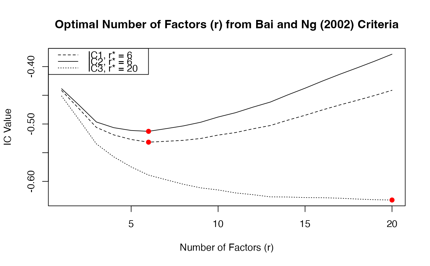
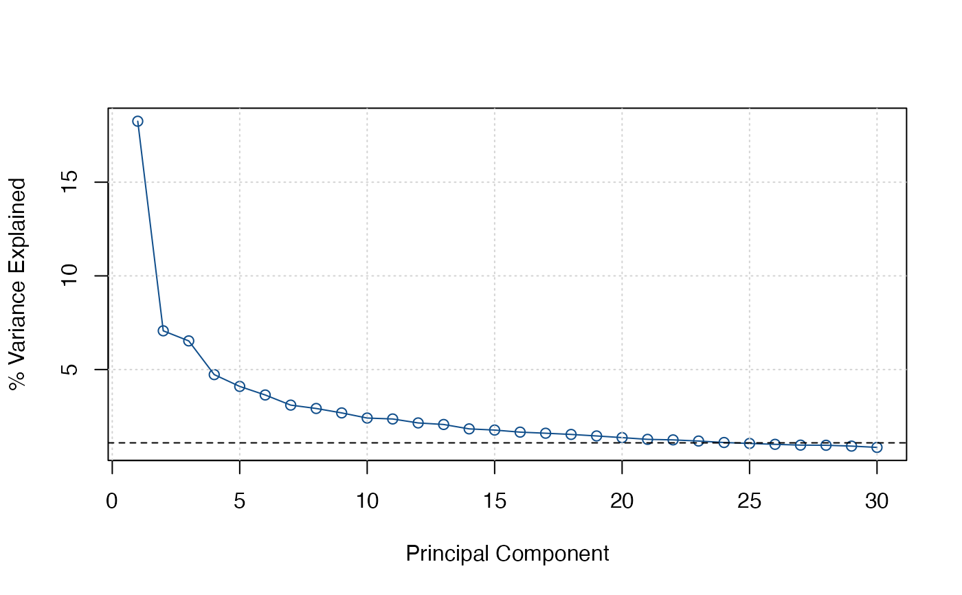
Information Criteria to Determine the Number of Factors (r)

Minimizes 3 information criteria proposed by Bai and Ng (2002) to determine the optimal number of factors r* to be used in an approximate factor model. A Screeplot can also be computed to eyeball the number of factors in the spirit of Onatski (2010).

Usage

ICr(X, max.r = min(20, ncol(X) - 1))

# S3 method for class 'ICr'
print(x, ...)

# S3 method for class 'ICr'
plot(x, ...)

# S3 method for class 'ICr'
screeplot(x, type = "pve", show.grid = TRUE, max.r = 30, ...)

Arguments

X: a T x n numeric data matrix or frame of stationary time series.
max.r: integer. The maximum number of factors for which IC should be computed (or eigenvalues to be displayed in the screeplot).
x: an object of type 'ICr'.
...: further arguments to ts.plot or plot.
type: character. Either "ev" (eigenvalues), "pve" (percent variance explained), or "cum.pve" (cumulative PVE). Multiple plots can be requested.
show.grid: logical. TRUE shows gridlines in each plot.

Value

A list of 4 elements:

F_pca: T x n matrix of principle component factor estimates.
eigenvalues: the eigenvalues of the covariance matrix of X.
IC: r.max x 3 'table' containing the 3 information criteria of Bai and Ng (2002), computed for all values of r from 1:r.max.
r.star: vector of length 3 containing the number of factors (r) minimizing each information criterion.

Details

Following Bai and Ng (2002) and De Valk et al. (2019), let $NSSR(r)$ be the normalized sum of squared residuals $SSR(r) / (n \times T)$ when r factors are estimated using principal components. Then the information criteria can be written as follows:

$$IC_{r1} = \ln(NSSR(r)) + r\left(\frac{n + T}{nT}\right) + \ln\left(\frac{nT}{n + T}\right)$$ $$IC_{r2} = \ln(NSSR(r)) + r\left(\frac{n + T}{nT}\right) + \ln(\min(n, T))$$ $$IC_{r3} = \ln(NSSR(r)) + r\left(\frac{\ln(\min(n, T))}{\min(n, T)}\right)$$

The optimal number of factors r* corresponds to the minimum IC. The three criteria are are asymptotically equivalent, but may give significantly different results for finite samples. The penalty in $IC_{r2}$ is highest in finite samples.

In the Screeplot a horizontal dashed line is shown signifying an eigenvalue of 1, or a share of variance corresponding to 1 divided by the number of eigenvalues.

Note

To determine the number of lags (p) in the factor transition equation, use the function vars::VARselect with r* principle components (also returned by ICr).

References

Bai, J., Ng, S. (2002). Determining the Number of Factors in Approximate Factor Models. Econometrica, 70(1), 191-221. https://doi.org/10.1111/1468-0262.00273.

Onatski, A. (2010). Determining the number of factors from empirical distribution of eigenvalues. The Review of Economics and Statistics, 92(4), 1004-1016.

De Valk, S., de Mattos, D., & Ferreira, P. (2019). Nowcasting: An R package for predicting economic variables using dynamic factor models. The R Journal, 11(1), 230-244.

Examples

library(xts)
library(vars)

ics <- ICr(diff(BM14_M))
#> Missing values detected: imputing data with tsnarmimp() with default settings
print(ics)
#> Optimal Number of Factors (r) from Bai and Ng (2002) Criteria
#> 
#> IC1 IC2 IC3 
#>   6   6  20 
plot(ics)

screeplot(ics)


# Optimal lag-order with 6 factors chosen
VARselect(ics$F_pca[, 1:6])
#> $selection
#> AIC(n)  HQ(n)  SC(n) FPE(n) 
#>      6      3      1      6 
#> 
#> $criteria
#>                  1          2          3          4          5          6
#> AIC(n)    6.916814   6.660193   6.426226   6.303207   6.254268   6.240250
#> HQ(n)     7.102739   7.005481   6.930879   6.967224   7.077649   7.222994
#> SC(n)     7.383723   7.527309   7.693550   7.970738   8.322007   8.708196
#> FPE(n) 1009.133494 780.867151 618.248189 547.148594 521.734680 515.519358
#>                 7          8          9         10
#> AIC(n)   6.332960   6.342459   6.365012   6.447964
#> HQ(n)    7.475069   7.643931   7.825849   8.068165
#> SC(n)    9.201114   9.610820  10.033580  10.516740
#> FPE(n) 567.198946 574.763323 590.710534 645.677979
#>