A dataset containing 14,358 raw network segments representing intersected road routes
between African cities. Each segment is defined by start and end coordinates with
aggregate importance metrics. This dataset is provided to demonstrate how package
functions like consolidate_graph() and
simplify_network() can process messy segment data
into clean analytical networks like africa_network.
Usage
data(africa_segments)Format
A data frame with 14,358 rows and 7 columns:
- FX
Numeric. Start point longitude (range: -17.4 to 49.2).
- FY
Numeric. Start point latitude (range: -34.2 to 37.2).
- TX
Numeric. End point longitude (range: -17.0 to 49.1).
- TY
Numeric. End point latitude (range: -34.2 to 37.2).
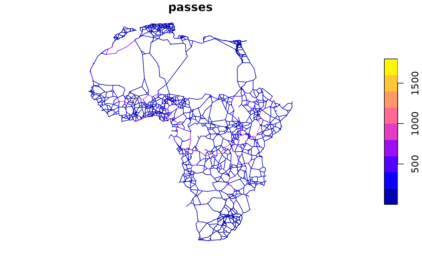
- passes
Integer. Number of optimal inter-city routes passing through this segment. Range: 1 to 1,615, median: 46.
- gravity
Numeric. Sum of population gravity weights from routes using this segment. Computed as sum of (pop_origin * pop_destination / spherical_distance_km) / 1e9.
- gravity_rd
Numeric. Sum of road-distance-weighted gravity from routes. Computed as sum of (pop_origin * pop_destination / road_distance_m) / 1e9.
Source
Derived from OpenStreetMap routing data via OSRM, processed through route intersection and aggregation.
Dataset constructed for: Krantz, S. (2024). Optimal Investments in Africa's Road Network. Policy Research Working Paper 10893. World Bank. doi:10.1596/1813-9450-10893 . Replication materials: https://github.com/SebKrantz/OptimalAfricanRoads.
Details
This dataset represents an intermediate stage in network construction, after routes have been
intersected but before network simplification. The segments have been simplified using
linestrings_from_graph() to retain only start and end coordinates.
The segments can be used to demonstrate the flownet network processing workflow:
Convert segments to an sf LINESTRING object using
linestrings_from_graph()Apply
consolidate_graph()to merge nearby nodesApply
simplify_network()to remove intermediate nodes
The passes field indicates how many optimal city-to-city routes use each segment,
serving as a measure of segment importance in the network. Higher values indicate
segments that are critical for efficient inter-city connectivity.
Examples
data(africa_segments)
head(africa_segments)
#>          FX       FY        TX       TY passes  gravity gravity_rd
#> 1 -17.44759 14.69386 -17.04861 14.70538     59 93.20669  67.218731
#> 2 -17.44759 14.69386 -16.70998 14.40844      6 59.98582  45.491608
#> 3 -17.04861 14.70538 -16.70998 14.40844     48 61.68941  42.121072
#> 4 -17.04861 14.70538 -16.96602 14.72614     11 31.51728  25.097660
#> 5 -17.03345 20.93362 -16.89503 21.28569     63  4.09779   2.981159
#> 6 -16.96602 14.72614 -16.63849 15.11222     10 20.13822  14.737626

# Summary statistics
summary(africa_segments[, c("passes", "gravity", "gravity_rd")])
#>      passes          gravity            gravity_rd
#>  Min.   :   1.0   Min.   :   0.0001   Min.   :   0.0001
#>  1st Qu.:  14.0   1st Qu.:   3.9964   1st Qu.:   2.8740
#>  Median :  46.0   Median :  16.5966   Median :  11.4518
#>  Mean   : 113.9   Mean   :  76.2857   Mean   :  53.9421
#>  3rd Qu.: 131.0   3rd Qu.:  64.4550   3rd Qu.:  43.4980
#>  Max.   :1615.0   Max.   :4144.5363   Max.   :3278.1380

# Segments with highest traffic
africa_segments[order(-africa_segments$passes), ][1:10, ]
#>             FX       FY       TX       TY passes  gravity gravity_rd
#> 672   -0.43130 12.19363 -0.35795 12.18282   1615 654.6566   483.7826
#> 5829  -1.52978 12.36658 -1.52187 12.37092   1584 646.9655   478.4648
#> 5830  -1.52187 12.37092 -1.51004 12.37915   1584 646.9655   478.4648
#> 649   -1.36024 12.43948 -1.26867 12.48558   1581 649.2992   480.4201
#> 651   -1.26432 12.48681 -0.43130 12.19363   1574 645.7477   477.1712
#> 647   -1.44519 12.39922 -1.37384 12.43304   1570 646.5881   478.1731
#> 641   -1.53359 12.36966 -1.52978 12.36658   1536 584.3362   435.5978
#> 5713  -2.01904 12.19641 -1.75856 12.23416   1437 564.3777   415.2477
#> 5714  -1.75503 12.23701 -1.63531 12.32471   1437 564.3777   415.2477
#> 13627 35.69371 -0.15936 35.70070 -0.16562   1395 496.1546   353.6817

# \donttest{
# Convert to sf and plot
library(sf)
segments_sf <- linestrings_from_graph(africa_segments)
plot(segments_sf["passes"])

# }
# }