Data Frame Based Objects

The three major data frame based classes in R are the base R data.frame, the data.table and the tibble, for which there also exists grouped (dplyr) and time based (tsibble, tibbletime) versions. Additional notable classes are the panel data frame (plm) and the spatial features data frame (sf).

For the former three collapse offer extremely fast and versatile converters qDF, qDT and qTBL that can be used to turn many R objects into data.frame’s, data.table’s or tibble’s, respectively:

library(collapse); library(data.table); library(tibble)
options(datatable.print.nrows = 10, 
        datatable.print.topn = 2)

identical(qDF(mtcars), mtcars)
## [1] TRUE

mtcarsDT <- qDT(mtcars, row.names.col = "car")
mtcarsDT
##               car  mpg cyl disp  hp drat    wt  qsec vs am gear carb
##  1:     Mazda RX4 21.0   6  160 110 3.90 2.620 16.46  0  1    4    4
##  2: Mazda RX4 Wag 21.0   6  160 110 3.90 2.875 17.02  0  1    4    4
## ---                                                                 
## 31: Maserati Bora 15.0   8  301 335 3.54 3.570 14.60  0  1    5    8
## 32:    Volvo 142E 21.4   4  121 109 4.11 2.780 18.60  1  1    4    2

mtcarsTBL <- qTBL(mtcars, row.names.col = "car")
print(mtcarsTBL, n = 3)
## # A tibble: 32 x 12
##   car             mpg   cyl  disp    hp  drat    wt  qsec    vs    am  gear  carb
##   <chr>         <dbl> <dbl> <dbl> <dbl> <dbl> <dbl> <dbl> <dbl> <dbl> <dbl> <dbl>
## 1 Mazda RX4      21       6   160   110  3.9   2.62  16.5     0     1     4     4
## 2 Mazda RX4 Wag  21       6   160   110  3.9   2.88  17.0     0     1     4     4
## 3 Datsun 710     22.8     4   108    93  3.85  2.32  18.6     1     1     4     1
## # ... with 29 more rows

These objects can then be manipulated using an advanced and attribute preserving set of (S3 generic) statistical and data manipulation functions. The following infographic summarizes the core collapse namespace:

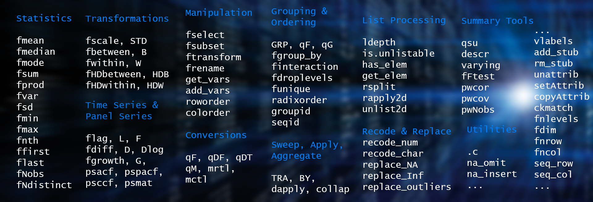
More details are provided in the freshly released cheat sheet, and further in the documentation and vignettes.

The statistical functions internally handle grouped and / or weighted computations on vectors, matrices and data frames, and seek to keep the attributes of the object.

# Simple data frame: Grouped mean by cyl -> groups = row.names  
fmean(fselect(mtcars, mpg, disp, drat), g = mtcars$cyl)
##        mpg     disp     drat
## 4 26.66364 105.1364 4.070909
## 6 19.74286 183.3143 3.585714
## 8 15.10000 353.1000 3.229286

With fgroup_by, collapse also introduces a fast grouping mechanism that works together with grouped_df versions of all statistical and transformation functions:

# Using Pipe operators and grouped data frames
library(magrittr)
mtcars %>% fgroup_by(cyl) %>% 
  fselect(mpg, disp, drat, wt) %>% fmean  
##   cyl      mpg     disp     drat       wt
## 1   4 26.66364 105.1364 4.070909 2.285727
## 2   6 19.74286 183.3143 3.585714 3.117143
## 3   8 15.10000 353.1000 3.229286 3.999214

# This is still a data.table 
mtcarsDT %>% fgroup_by(cyl) %>% 
  fselect(mpg, disp, drat, wt) %>% fmean
##    cyl      mpg     disp     drat       wt
## 1:   4 26.66364 105.1364 4.070909 2.285727
## 2:   6 19.74286 183.3143 3.585714 3.117143
## 3:   8 15.10000 353.1000 3.229286 3.999214

# Same with tibble: here computing weighted group means -> also saves sum of weights in each group
mtcarsTBL %>% fgroup_by(cyl) %>% 
  fselect(mpg, disp, drat, wt) %>% fmean(wt)
## # A tibble: 3 x 5
##     cyl sum.wt   mpg  disp  drat
##   <dbl>  <dbl> <dbl> <dbl> <dbl>
## 1     4   25.1  25.9  110.  4.03
## 2     6   21.8  19.6  185.  3.57
## 3     8   56.0  14.8  362.  3.21

A specialty of the grouping mechanism is that it fully preserves the structure / attributes of the object, and thus permits the creation of a grouped version of any data frame like object.

# This created a grouped data.table
gmtcarsDT <- mtcarsDT %>% fgroup_by(cyl)
gmtcarsDT
##               car  mpg cyl disp  hp drat    wt  qsec vs am gear carb
##  1:     Mazda RX4 21.0   6  160 110 3.90 2.620 16.46  0  1    4    4
##  2: Mazda RX4 Wag 21.0   6  160 110 3.90 2.875 17.02  0  1    4    4
## ---                                                                 
## 31: Maserati Bora 15.0   8  301 335 3.54 3.570 14.60  0  1    5    8
## 32:    Volvo 142E 21.4   4  121 109 4.11 2.780 18.60  1  1    4    2
## 
## Grouped by:  cyl  [3 | 11 (3.5)]
# The print shows: [N. groups | Avg. group size (SD around avg. group size)]

# Subsetting drops groups 
gmtcarsDT[1:2]
##              car mpg cyl disp  hp drat    wt  qsec vs am gear carb
## 1:     Mazda RX4  21   6  160 110  3.9 2.620 16.46  0  1    4    4
## 2: Mazda RX4 Wag  21   6  160 110  3.9 2.875 17.02  0  1    4    4

# Any class-specific methods are independent of the attached groups
gmtcarsDT[, new := mean(mpg)]
gmtcarsDT[, lapply(.SD, mean), by = vs, .SDcols = -1L] # Again groups are dropped
##    vs      mpg      cyl     disp        hp     drat       wt     qsec        am     gear     carb
## 1:  0 16.61667 7.444444 307.1500 189.72222 3.392222 3.688556 16.69389 0.3333333 3.555556 3.611111
## 2:  1 24.55714 4.571429 132.4571  91.35714 3.859286 2.611286 19.33357 0.5000000 3.857143 1.785714
##         new
## 1: 20.09062
## 2: 20.09062

# Groups are always preserved in column-subsetting operations
gmtcarsDT[, 9:13] 
##     vs am gear carb      new
##  1:  0  1    4    4 20.09062
##  2:  0  1    4    4 20.09062
## ---                         
## 31:  0  1    5    8 20.09062
## 32:  1  1    4    2 20.09062
## 
## Grouped by:  cyl  [3 | 11 (3.5)]

The grouping is also dropped in aggregations, but preserved in transformations keeping data dimensions:

# Grouped medians 
fmedian(gmtcarsDT[, 9:13])
##    cyl vs am gear carb      new
## 1:   4  1  1    4  2.0 20.09062
## 2:   6  1  0    4  4.0 20.09062
## 3:   8  0  0    3  3.5 20.09062
# Note: unique grouping columns are stored in the attached grouping object 
# and added if keep.group_vars = TRUE (the default)

# Replacing data by grouped median (grouping columns are not selected and thus not present)
fmedian(gmtcarsDT[, 4:5], TRA = "replace")
##      disp    hp
##  1: 167.6 110.0
##  2: 167.6 110.0
## ---            
## 31: 350.5 192.5
## 32: 108.0  91.0
## 
## Grouped by:  cyl  [3 | 11 (3.5)]

# Weighted scaling and centering data (here also selecting grouping column)
mtcarsDT %>% fgroup_by(cyl) %>% 
  fselect(cyl, mpg, disp, drat, wt) %>% fscale(wt)
##     cyl    wt         mpg       disp      drat
##  1:   6 2.620  0.96916875 -0.6376553 0.7123846
##  2:   6 2.875  0.96916875 -0.6376553 0.7123846
## ---                                           
## 31:   8 3.570  0.07335466 -0.8685527 0.9844833
## 32:   4 2.780 -1.06076989  0.3997723 0.2400387
## 
## Grouped by:  cyl  [3 | 11 (3.5)]

As mentioned, this works for any data frame like object, even a suitable list:

# Here computing a weighted grouped standard deviation
as.list(mtcars) %>% fgroup_by(cyl, vs, am) %>% 
  fsd(wt) %>% str
## List of 11
##  $ cyl   : num [1:7] 4 4 4 6 6 8 8
##  $ vs    : num [1:7] 0 1 1 0 1 0 0
##  $ am    : num [1:7] 1 0 1 1 0 0 1
##  $ sum.wt: num [1:7] 2.14 8.8 14.2 8.27 13.55 ...
##  $ mpg   : num [1:7] 0 1.236 4.833 0.655 1.448 ...
##  $ disp  : num [1:7] 0 11.6 19.25 7.55 39.93 ...
##  $ hp    : num [1:7] 0 17.3 22.7 32.7 8.3 ...
##  $ drat  : num [1:7] 0 0.115 0.33 0.141 0.535 ...
##  $ qsec  : num [1:7] 0 1.474 0.825 0.676 0.74 ...
##  $ gear  : num [1:7] 0 0.477 0.32 0.503 0.519 ...
##  $ carb  : num [1:7] 0 0.477 0.511 1.007 1.558 ...
##  - attr(*, "row.names")= int [1:7] 1 2 3 4 5 6 7

The function fungroup can be used to undo any grouping operation.

identical(mtcarsDT,
          mtcarsDT %>% fgroup_by(cyl, vs, am) %>% fungroup)
## [1] TRUE

Apart from the grouping mechanism with fgroup_by, which is very fast and versatile, collapse also supports regular grouped tibbles created with dplyr:

library(dplyr)
# Same as summarize_all(sum) and considerably faster
mtcars %>% group_by(cyl) %>% fsum
## # A tibble: 3 x 11
##     cyl   mpg  disp    hp  drat    wt  qsec    vs    am  gear  carb
##   <dbl> <dbl> <dbl> <dbl> <dbl> <dbl> <dbl> <dbl> <dbl> <dbl> <dbl>
## 1     4  293. 1157.   909  44.8  25.1  211.    10     8    45    17
## 2     6  138. 1283.   856  25.1  21.8  126.     4     3    27    24
## 3     8  211. 4943.  2929  45.2  56.0  235.     0     2    46    49

# Same as muatate_all(sum)
mtcars %>% group_by(cyl) %>% fsum(TRA = "replace_fill") %>% head(3)
## # A tibble: 3 x 11
## # Groups:   cyl [2]
##     cyl   mpg  disp    hp  drat    wt  qsec    vs    am  gear  carb
##   <dbl> <dbl> <dbl> <dbl> <dbl> <dbl> <dbl> <dbl> <dbl> <dbl> <dbl>
## 1     6  138. 1283.   856  25.1  21.8  126.     4     3    27    24
## 2     6  138. 1283.   856  25.1  21.8  126.     4     3    27    24
## 3     4  293. 1157.   909  44.8  25.1  211.    10     8    45    17

One major goal of the package is to make R suitable for (large) panel data, thus collapse also supports panel-data.frames created with the plm package:

library(plm)
pwlddev <- pdata.frame(wlddev, index = c("iso3c", "year"))

# Centering (within-transforming) columns 9-12 using the within operator W()
head(W(pwlddev, cols = 9:12), 3)
##          iso3c year W.PCGDP  W.LIFEEX W.GINI W.ODA
## ABW-1960   ABW 1960      NA -6.547351     NA    NA
## ABW-1961   ABW 1961      NA -6.135351     NA    NA
## ABW-1962   ABW 1962      NA -5.765351     NA    NA

# Computing growth rates of columns 9-12 using the growth operator G()
head(G(pwlddev, cols = 9:12), 3)
##          iso3c year G1.PCGDP G1.LIFEEX G1.GINI G1.ODA
## ABW-1960   ABW 1960       NA        NA      NA     NA
## ABW-1961   ABW 1961       NA 0.6274558      NA     NA
## ABW-1962   ABW 1962       NA 0.5599782      NA     NA

Perhaps a note about operators is necessary here before proceeding: collapse offers a set of transformation operators for its vector-valued fast functions:

# Operators
.OPERATOR_FUN
##  [1] "STD"  "B"    "W"    "HDB"  "HDW"  "L"    "F"    "D"    "Dlog" "G"

# Corresponding (programmers) functions
setdiff(.FAST_FUN, .FAST_STAT_FUN)
## [1] "fscale"     "fbetween"   "fwithin"    "fHDbetween" "fHDwithin"  "flag"       "fdiff"     
## [8] "fgrowth"

These operators are principally just function shortcuts that exist for parsimony and in-formula use (e.g. to specify dynamic or fixed effects models using lm(), see the documentation). They however also have some useful extra features in the data.frame method, such as internal column-subsetting using the cols argument or stub-renaming transformed columns (adding a ‘W.’ or ‘Gn.’ prefix as shown above). They also permit grouping variables to be passed using formulas, including options to keep (default) or drop those variables in the output. We will see this feature when using time series below.

To round things off for data frames, I demonstrate the use of collapse with classes it was not directly built to support but can also handle very well. Through it’s built in capabilities for handling panel data, tsibble’s can seamlessly be utilized:

library(tsibble)
tsib <- as_tsibble(EuStockMarkets)

# Computing daily and annual growth rates on tsibble
head(G(tsib, c(1, 260), by = ~ key, t = ~ index), 3)
## # A tsibble: 3 x 4 [1s] <UTC>
## # Key:       key [1]
##   key   index               G1.value L260G1.value
##   <chr> <dttm>                 <dbl>        <dbl>
## 1 DAX   1991-07-01 02:18:33   NA               NA
## 2 DAX   1991-07-02 12:00:00   -0.928           NA
## 3 DAX   1991-07-03 21:41:27   -0.441           NA

# Computing a compounded annual growth rate
head(G(tsib, 260, by = ~ key, t = ~ index, power = 1/260), 3)
## # A tsibble: 3 x 3 [1s] <UTC>
## # Key:       key [1]
##   key   index               L260G1.value
##   <chr> <dttm>                     <dbl>
## 1 DAX   1991-07-01 02:18:33           NA
## 2 DAX   1991-07-02 12:00:00           NA
## 3 DAX   1991-07-03 21:41:27           NA

Similarly for tibbletime:

library(tibbletime); library(tsbox)
# Using the tsbox converter
tibtm <- ts_tibbletime(EuStockMarkets)

# Computing daily and annual growth rates on tibbletime
head(G(tibtm, c(1, 260), t = ~ time), 3)
## # A time tibble: 3 x 9
## # Index: time
##   time                G1.DAX L260G1.DAX G1.SMI L260G1.SMI G1.CAC L260G1.CAC G1.FTSE L260G1.FTSE
##   <dttm>               <dbl>      <dbl>  <dbl>      <dbl>  <dbl>      <dbl>   <dbl>       <dbl>
## 1 1991-07-01 02:18:27 NA             NA NA             NA  NA            NA  NA              NA
## 2 1991-07-02 12:01:32 -0.928         NA  0.620         NA  -1.26         NA   0.679          NA
## 3 1991-07-03 21:44:38 -0.441         NA -0.586         NA  -1.86         NA  -0.488          NA
# ...

Finally lets consider the simple features data frame:

library(sf)
nc <- st_read(system.file("shape/nc.shp", package="sf"))
## Reading layer `nc' from data source `C:\Users\Sebastian Krantz\Documents\R\win-library\4.0\sf\shape\nc.shp' using driver `ESRI Shapefile'
## Simple feature collection with 100 features and 14 fields
## geometry type:  MULTIPOLYGON
## dimension:      XY
## bbox:           xmin: -84.32385 ymin: 33.88199 xmax: -75.45698 ymax: 36.58965
## geographic CRS: NAD27

# Fast selecting columns (need to add 'geometry' column to not break the class)
plot(fselect(nc, AREA, geometry))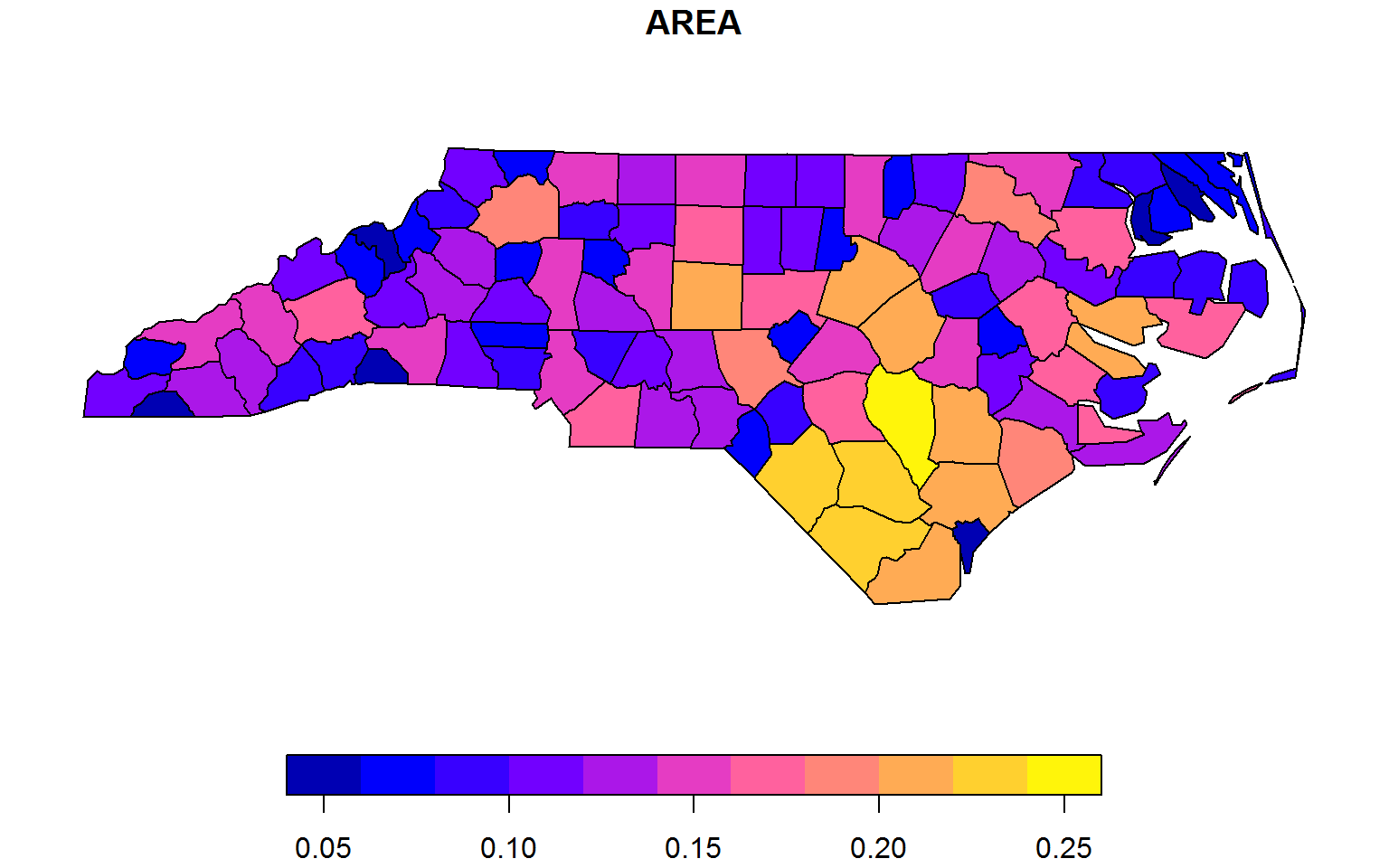

# Subsetting 
fsubset(nc, AREA > 0.23, NAME, AREA, geometry)
## Simple feature collection with 3 features and 2 fields
## geometry type:  MULTIPOLYGON
## dimension:      XY
## bbox:           xmin: -84.32385 ymin: 33.88199 xmax: -75.45698 ymax: 36.58965
## geographic CRS: NAD27
##       NAME  AREA                       geometry
## 1  Sampson 0.241 MULTIPOLYGON (((-78.11377 3...
## 2  Robeson 0.240 MULTIPOLYGON (((-78.86451 3...
## 3 Columbus 0.240 MULTIPOLYGON (((-78.65572 3...

# Standardizing numeric columns (by reference)
settransformv(nc, is.numeric, STD, apply = FALSE)
# Note: Here using using operator STD() instead of fscale() to stub-rename standardized columns.
# apply = FALSE uses STD.data.frame on all numeric columns instead of lapply(data, STD)
head(nc, 2)
## Simple feature collection with 2 features and 26 fields
## geometry type:  MULTIPOLYGON
## dimension:      XY
## bbox:           xmin: -81.74107 ymin: 36.23436 xmax: -80.90344 ymax: 36.58965
## geographic CRS: NAD27
##    AREA PERIMETER CNTY_ CNTY_ID      NAME  FIPS FIPSNO CRESS_ID BIR74 SID74 NWBIR74 BIR79 SID79
## 1 0.114     1.442  1825    1825      Ashe 37009  37009        5  1091     1      10  1364     0
## 2 0.061     1.231  1827    1827 Alleghany 37005  37005        3   487     0      10   542     3
##   NWBIR79                       geometry  STD.AREA STD.PERIMETER STD.CNTY_ STD.CNTY_ID STD.FIPSNO
## 1      19 MULTIPOLYGON (((-81.47276 3... -0.249186    -0.4788595 -1.511125   -1.511125  -1.568344
## 2      12 MULTIPOLYGON (((-81.23989 3... -1.326418    -0.9163351 -1.492349   -1.492349  -1.637282
##   STD.CRESS_ID  STD.BIR74  STD.SID74 STD.NWBIR74  STD.BIR79  STD.SID79 STD.NWBIR79
## 1    -1.568344 -0.5739411 -0.7286824  -0.7263602 -0.5521659 -0.8863574  -0.6750055
## 2    -1.637282 -0.7308990 -0.8571979  -0.7263602 -0.7108697 -0.5682866  -0.6785480

Matrix Based Objects

collapse also offers a converter qM to efficiently convert various objects to matrix:

m <- qM(mtcars)

Grouped and / or weighted computations and transformations work as with with data frames:

# Grouped means
fmean(m, g = mtcars$cyl)
##        mpg cyl     disp        hp     drat       wt     qsec        vs        am     gear     carb
## 4 26.66364   4 105.1364  82.63636 4.070909 2.285727 19.13727 0.9090909 0.7272727 4.090909 1.545455
## 6 19.74286   6 183.3143 122.28571 3.585714 3.117143 17.97714 0.5714286 0.4285714 3.857143 3.428571
## 8 15.10000   8 353.1000 209.21429 3.229286 3.999214 16.77214 0.0000000 0.1428571 3.285714 3.500000

# Grouped and weighted standardizing
head(fscale(m, g = mtcars$cyl, w = mtcars$wt), 3)
##                      mpg cyl        disp         hp       drat         wt       qsec         vs
## Mazda RX4      0.9691687 NaN -0.63765527 -0.5263758  0.7123846 -1.6085211 -1.0438559 -1.2509539
## Mazda RX4 Wag  0.9691687 NaN -0.63765527 -0.5263758  0.7123846 -0.8376064 -0.6921302 -1.2509539
## Datsun 710    -0.7333024 NaN -0.08822497  0.4896429 -0.5526066 -0.1688057 -0.4488514  0.2988833
##                     am        gear      carb
## Mazda RX4     1.250954  0.27612029  0.386125
## Mazda RX4 Wag 1.250954  0.27612029  0.386125
## Datsun 710    0.719370 -0.09429567 -1.133397

Various matrix-based time series classes such as xts / zoo and timeSeries are also easily handled:

# ts / mts
# Note: G() by default renames the columns, fgrowth() does not
plot(G(EuStockMarkets))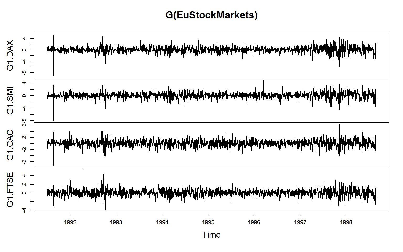

# xts
library(xts) 
ESM_xts <- ts_xts(EuStockMarkets) # using tsbox::ts_xts
head(G(ESM_xts), 3)
##                         G1.DAX     G1.SMI    G1.CAC    G1.FTSE
## 1991-07-01 02:18:27         NA         NA        NA         NA
## 1991-07-02 12:01:32 -0.9283193  0.6197485 -1.257897  0.6793256
## 1991-07-03 21:44:38 -0.4412412 -0.5863192 -1.856612 -0.4877652

plot(G(ESM_xts), legend.loc = "bottomleft")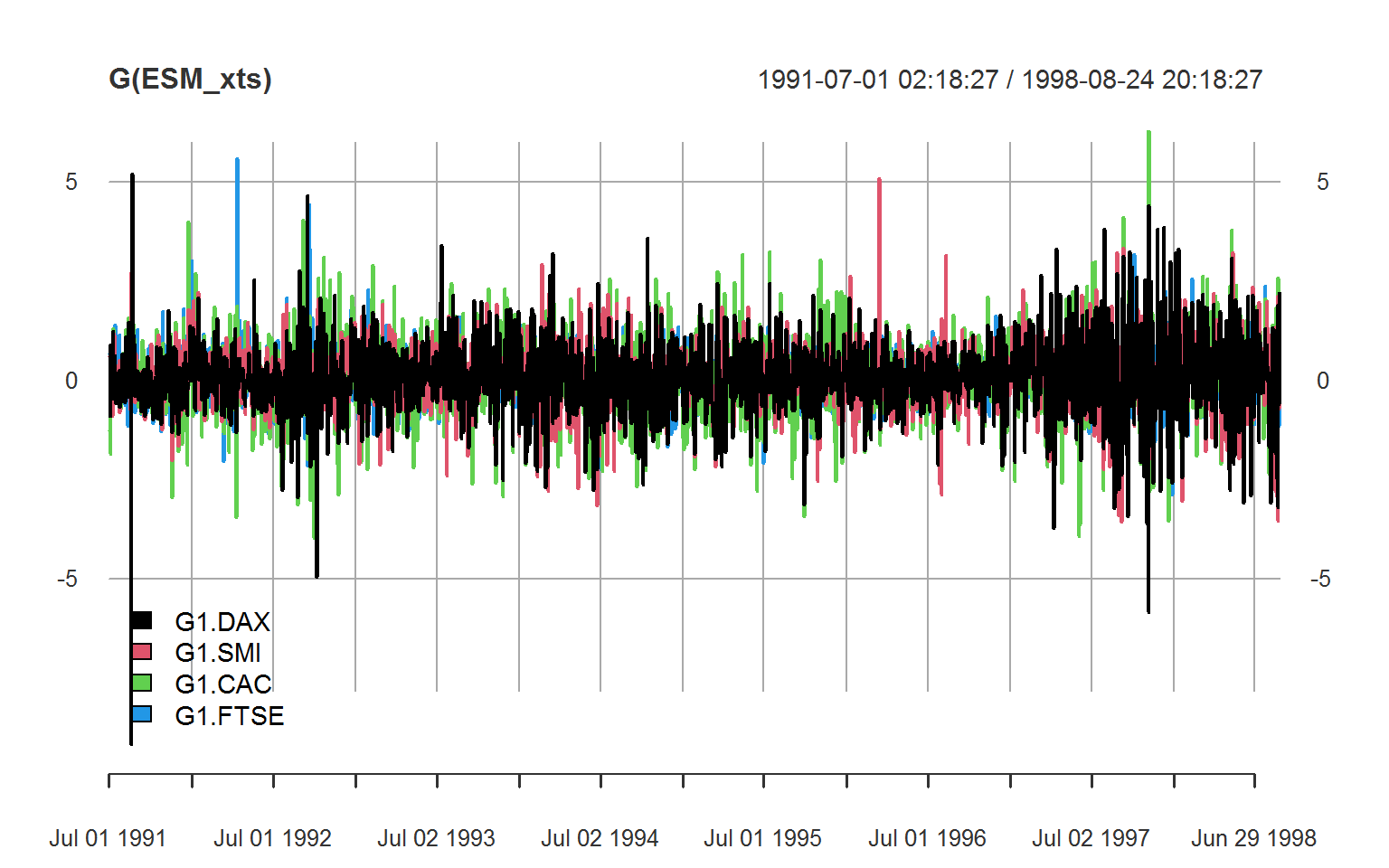

# timeSeries
library(timeSeries) # using tsbox::ts_timeSeries
ESM_timeSeries <- ts_timeSeries(EuStockMarkets)
# Note: G() here also renames the columns but the names of the series are also stored in an attribute
head(G(ESM_timeSeries), 3)
## GMT
##                            DAX        SMI       CAC       FTSE
## 1991-06-30 23:18:27         NA         NA        NA         NA
## 1991-07-02 09:01:32 -0.9283193  0.6197485 -1.257897  0.6793256
## 1991-07-03 18:44:38 -0.4412412 -0.5863192 -1.856612 -0.4877652

plot(G(ESM_timeSeries), plot.type = "single", at = "pretty")
legend("bottomleft", colnames(G(qM(ESM_timeSeries))), lty = 1, col = 1:4)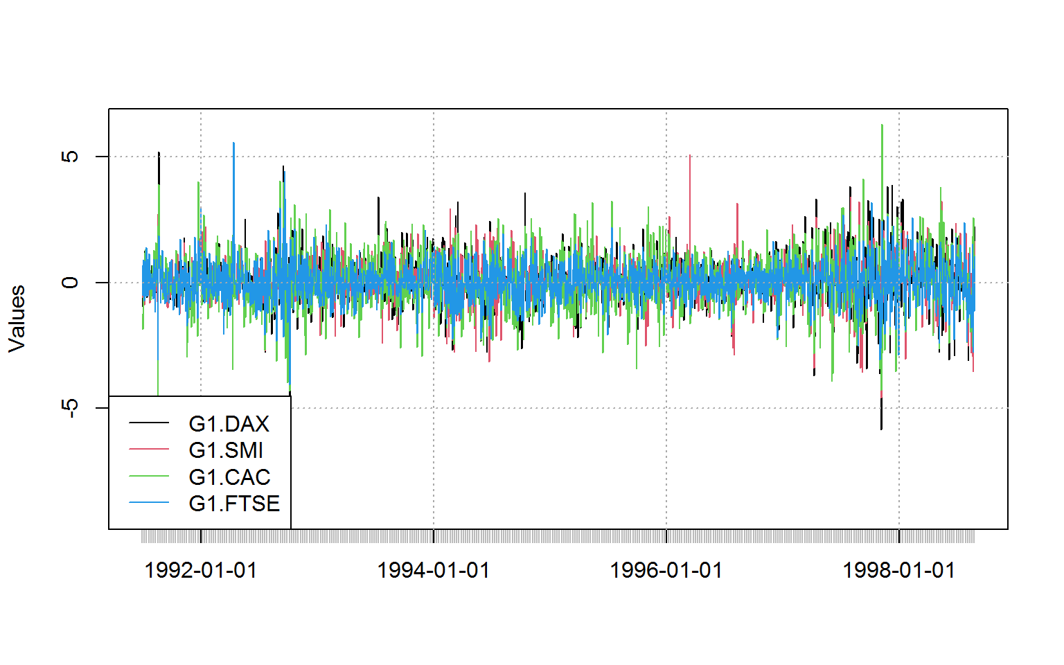

Aggregating these objects yields a plain matrix with groups in the row-names:

# Aggregating by year: creates plain matrix with row-names (g is second argument)
EuStockMarkets %>% fmedian(round(time(.)))
##           DAX     SMI    CAC    FTSE
## 1991 1628.750 1678.10 1772.8 2443.60
## 1992 1649.550 1733.30 1863.5 2558.50
## 1993 1606.640 2061.70 1837.5 2773.40
## 1994 2089.770 2727.10 2148.0 3111.40
## 1995 2072.680 2591.60 1918.5 3091.70
## 1996 2291.820 3251.60 1946.2 3661.65
## 1997 2861.240 3906.55 2297.1 4075.35
## 1998 4278.725 6077.40 3002.7 5222.20
## 1999 5905.150 8102.70 4205.4 5884.50

# Same thing with the other objects
all_obj_equal(ESM_xts %>% fmedian(substr(time(.), 1L, 4L)),
              ESM_timeSeries %>% fmedian(substr(time(.), 1L, 4L)))
## [1] TRUE

Benchmarks

Extensive benchmarks and examples against native dplyr / tibble and plm are provided here and here, making it evident that collapse provides both greater versatility and massive performance improvements over the methods defined for these objects. Benchmarks against data.table were provided in a previous post, where collapse compared favorably on a 2-core machine (particularly for weighted and := type operations). In general collapse functions are extremely well optimized, with basic execution speeds below 30 microseconds, and efficiently scale to larger operations. Most importantly, they preserve the data structure and attributes (including column attributes) of the objects passed to them. They also efficiently skip missing values and avoid some of the undesirable behavior endemic of base R¹.

Here I will add to the above resources just a small benchmark to prove that computations with collapse are also faster than any native methods and suggested programming principles for the various time series classes:

library(dplyr) # needed for tibbletime / tsibble comparison    
library(microbenchmark)

# Computing the first difference
microbenchmark(ts = diff(EuStockMarkets),
               collapse_ts = fdiff(EuStockMarkets),
               xts = diff(ESM_xts),
               collapse_xts = fdiff(ESM_xts),
               timeSeries = diff(ESM_timeSeries),
               collapse_timeSeries = fdiff(ESM_timeSeries),
               # taking difference function from tsibble
               dplyr_tibbletime = mutate_at(tibtm, 2:5, difference, order_by = tibtm$time),
               collapse_tibbletime_D = D(tibtm, t = ~ time),
               # collapse equivalent to the dplyr method (tfmv() abbreviates ftransformv())
               collapse_tibbletime_tfmv = tfmv(tibtm, 2:5, fdiff, t = time, apply = FALSE),
               # dplyr helpers provided by tsibble package
               dplyr_tsibble = mutate(group_by_key(tsib), value = difference(value, order_by = index)),
               collapse_tsibble_D = D(tsib, 1, 1, ~ key, ~ index),
               # Again we can do the same using collapse (tfm() abbreviates ftransform())
               collapse_tsibble_tfm = tfm(tsib, value = fdiff(value, 1, 1, key, index)))
## Unit: microseconds
##                      expr       min         lq       mean     median         uq        max neval cld
##                        ts  1681.018  2061.2220  2719.8758  2313.1290  3055.6870   9473.855   100  a 
##               collapse_ts    25.883    56.4505   163.3896    70.9540    88.1340   8732.636   100  a 
##                       xts    93.713   176.7150   279.5615   200.3655   257.0395   3656.561   100  a 
##              collapse_xts    42.840    78.0940   116.1231    99.7370   126.5120    597.973   100  a 
##                timeSeries  1964.386  2287.4700  3185.6565  2742.4210  3310.7180  17093.102   100  a 
##       collapse_timeSeries    52.658    93.9355  2483.3061   108.4390   132.7590 235259.074   100  a 
##          dplyr_tibbletime  8097.625 10173.1265 14784.9888 11176.0700 12863.3355 239144.113   100   b
##     collapse_tibbletime_D   568.967   630.5490   857.0829   751.2595   850.3270   8017.301   100  a 
##  collapse_tibbletime_tfmv   501.137   585.4780   773.2819   664.2410   817.0815   2922.035   100  a 
##             dplyr_tsibble 10386.434 12641.1040 14690.4243 13558.5910 15970.5640  32364.171   100   b
##        collapse_tsibble_D   963.897  1056.4935  1338.5404  1210.8955  1477.7525   3665.485   100  a 
##      collapse_tsibble_tfm   940.246   993.5720  1272.6027  1114.9525  1420.6320   6188.128   100  a

# Sequence of lagged/leaded and iterated differences (not supported by either of these methods)
head(fdiff(ESM_xts, -1:1, diff = 1:2)[, 1:6], 3) 
##                     FD1.DAX FD2.DAX     DAX D1.DAX D2.DAX FD1.SMI
## 1991-07-01 02:18:27   15.12    8.00 1628.75     NA     NA   -10.4
## 1991-07-02 12:01:32    7.12   21.65 1613.63 -15.12     NA     9.9
## 1991-07-03 21:44:38  -14.53  -17.41 1606.51  -7.12      8    -5.5
head(D(tibtm, -1:1, diff = 1:2, t = ~ time), 3)
## # A time tibble: 3 x 21
## # Index: time
##   time                FD1.DAX FD2.DAX   DAX D1.DAX D2.DAX FD1.SMI FD2.SMI   SMI D1.SMI D2.SMI FD1.CAC
##   <dttm>                <dbl>   <dbl> <dbl>  <dbl>  <dbl>   <dbl>   <dbl> <dbl>  <dbl>  <dbl>   <dbl>
## 1 1991-07-01 02:18:27   15.1     8.00 1629.  NA     NA      -10.4   -20.3 1678.   NA     NA      22.3
## 2 1991-07-02 12:01:32    7.12   21.7  1614. -15.1   NA        9.9    15.4 1688.   10.4   NA      32.5
## 3 1991-07-03 21:44:38  -14.5   -17.4  1607.  -7.12   8.00    -5.5    -3   1679.   -9.9  -20.3     9.9
## # ... with 9 more variables: FD2.CAC <dbl>, CAC <dbl>, D1.CAC <dbl>, D2.CAC <dbl>, FD1.FTSE <dbl>,
## #   FD2.FTSE <dbl>, FTSE <dbl>, D1.FTSE <dbl>, D2.FTSE <dbl>
head(D(tsib, -1:1, diff = 1:2, ~ key, ~ index), 3)
## # A tsibble: 3 x 7 [1s] <UTC>
## # Key:       key [1]
##   key   index               FD1.value FD2.value value D1.value D2.value
##   <chr> <dttm>                  <dbl>     <dbl> <dbl>    <dbl>    <dbl>
## 1 DAX   1991-07-01 02:18:33     15.1       8.00 1629.    NA       NA   
## 2 DAX   1991-07-02 12:00:00      7.12     21.7  1614.   -15.1     NA   
## 3 DAX   1991-07-03 21:41:27    -14.5     -17.4  1607.    -7.12     8.00

microbenchmark(collapse_xts = fdiff(ESM_xts, -1:1, diff = 1:2),
               collapse_tibbletime = D(tibtm, -1:1, diff = 1:2, t = ~ time),
               collapse_tsibble = D(tsib, -1:1, diff = 1:2, ~ key, ~ index))
## Unit: microseconds
##                 expr      min        lq      mean   median       uq       max neval cld
##         collapse_xts  147.263  218.2155  358.0477  254.362  290.508  8398.843   100 a  
##  collapse_tibbletime  750.144  988.4405 1348.9559 1026.149 1085.722 13947.942   100  b 
##     collapse_tsibble 1258.421 1653.3505 1793.5130 1707.793 1757.327  8411.784   100   c

Conclusion

This concludes this short demonstration. collapse is an advanced, fast and versatile data manipulation package. If you have followed until here I am convinced you will find it very useful, particularly if you are working in advanced statistics, econometrics, surveys, time series, panel data and the like, or if you care much about performance and non-destructive working in R. For more information about the package see the website, study the cheat sheet or call help("collapse-documentation") after install to bring up the built-in documentation.

Appendix: So how does this all actually work?

Statistical functions like fmean are S3 generic with user visible ‘default’, ‘matrix’ and ‘data.frame’ methods, and hidden ‘list’ and ‘grouped_df’ methods. Transformation functions like fwithin additionally have ‘pseries’ and ‘pdata.frame’ methods to support plm objects.

The ‘default’, ‘matrix’ and ‘data.frame’ methods handle object attributes intelligently. In the case of ‘data.frame’s’ only the ‘row.names’ attribute is modified accordingly, other attributes (including column attributes) are preserved. This also holds for data manipulation functions like fselect, fsubset, ftransform etc.. ‘default’ and ‘matrix’ methods preserve attributes as long as the data dimensions are kept.

In addition, the ‘default’ method checks if its argument is actually a matrix, and calls the matrix method if is.matrix(x) && !inherits(x, "matrix") is TRUE. This prevents classed matrix-based objects (such as xts time series) not inheriting from ‘matrix’ being handled by the default method.