![]()
I am excited to introduce a new R package called flownet providing high-performance tools for transport modeling—network processing, route enumeration, and traffic assignment in R. As of now, the package implements the Path-Sized Logit (PSL) model (Ben-Akiva and Bierlaire, 1999)—a powerful and well-established method for stochastic traffic assignment accounting for route overlap—alongside a novel route enumeration algorithm and a highly efficient All-or-Nothing assignment solution. Furthermore, it provides powerful utility functions for (multimodal) network processing, including recursive graph consolidation/contraction, and/or simplification. These features, combined with an accessible representation of graphs and (sparse) origin-destination (OD) matrices using data frames and a parsimonious API, make it a compelling toolbox for both transport analytics and graph manipulation.
As has come to be expected of my packages, flownet strives to be computationally efficient, building on a whole array of fastverse libraries including collapse and kit for fast data manipulation, igraph for efficient routing, geodist and leaderCluster for spatial distances and clustering, and mirai for efficient R-level parallelism. These dependencies are supplemented by custom C code, e.g., the PSL is implemented fully in C. There is still significant room for improvements, particularly if igraph can be replaced with internal C/C++ routing code, which could port the entire route enumeration algorithm to C/C++. Such innovation may be the subject of future updates, alongside new traffic assignment methods.
The package supports directed and undirected graphs and multimodal networks.1 In the following I demonstrate flownet on two networks:
The first is the African continental road network I built in my Job Market Paper. It is included in the package. This network is already consolidated and has 1379 nodes and 2344 edges representing 315,000 km of road network. It is thus a rather small network as far as the capabilities of flownet are concerned.
The second network is the US Freight Analysis Framework (FAF5) network comprising 487,384 links (edges) and 348,498 nodes. This network is very large and requires careful tuning of the PSL method. It also provides an excellent test case to demonstrate flownet’s network simplification capabilities.
Example 1: Africa’s Continental Road Network
The africa_network, taken from Krantz (2024) Optimal Investments in Africa’s Road Network, is included in the package. It was generated by intersecting and simplifying fastest OSRM car routes between 453 African cities with population > 100,000 and international ports—provided in africa_cities_ports. The procedure is described in the paper, and further demonstrated in the introductory vignette using flownet’s network processing tools. For this blog post we will take the network as given and defer the network processing workflow to the second (FAF5) example below.
The network includes 481 new links proposed by a network finding algorithm described in Section 4.2 of the paper. Below I plot the network with proposed links in grey and the 453 (port-)cities in black.
library(fastverse)
## -- Attaching packages ------------------------------------------------------------------------------------------------------------- fastverse 0.3.4 --
## v data.table 1.17.0     v kit        0.0.21
## v magrittr   2.0.4      v collapse   2.1.6
fastverse_extend(flownet, sf, tmap)
## -- Attaching extension packages --------------------------------------------------------------------------------------------------- fastverse 0.3.4 --
## v flownet 0.2.0      v tmap    4.2
## v sf      1.0.20
# Plot network colored by travel speed
tm_basemap("CartoDB.Positron", zoom = 4) +
tm_shape(africa_network) +
  tm_lines(col = "speed_kmh",
           col.scale = tm_scale_continuous(values = "turbo",
                                           values.range = c(0.1, 0.9),
                                           value.na = "grey"),
           col.legend = tm_legend("Speed (km/h)", position = c("left", "bottom"),
                                  frame = FALSE, text.size = 0.8, title.size = 1,
                                  item.height = 2, na.show = FALSE), lwd = 1.5) +
tm_shape(africa_cities_ports) + tm_dots(size = 0.1) +
tm_layout(frame = FALSE, outer.margins = 0)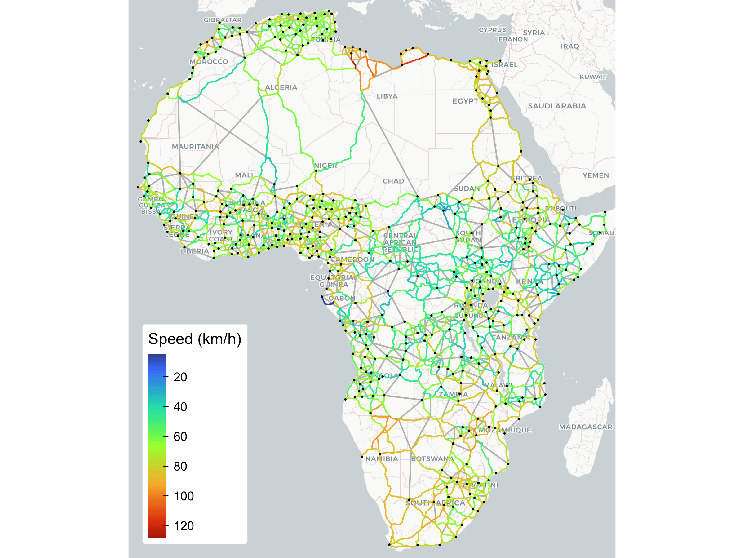
Evidently, OSRM link speeds differ widely, with speeds along many central African roads around 40km/h, and higher speeds closer to urban centers. Below, I further describe the network after removing the proposed links. As detailed in Section 3 of the paper, I extracted border and documentary times and costs of exporting and importing from the last World Bank Doing Business Survey (data collected in 2019), and converted them to travel-time-equivalent frictions (in minutes) along border-crossing links. There is thus a frictionless duration (travel time) variable and border_time (which includes documentary time—median 76h), which added together give the total_time needed to trade across a link.
# Removing potential new links
africa_net <- fsubset(africa_network, !add, -add)
names(africa_net) |> cat(sep = ", ")
## from, to, from_ctry, to_ctry, FX, FY, TX, TY, sp_distance, distance, duration, speed_kmh, passes, gravity, gravity_rd, border_dist, total_dist, border_time, total_time, duration_100kmh, total_time_100kmh, rugg, pop_wpop, pop_wpop_km2, cost_km, upgrade_cat, ug_cost_km, geometry
qsu(africa_net, cols = .c(from, to, speed_kmh, distance, duration, border_time, total_time))
##                 N       Mean          SD     Min         Max
## from         2344   669.4347    391.7331       1        1377
## to           2344   688.3921    395.8184       2        1379
## speed_kmh    2344    65.2302     16.0805  5.1429     127.749
## distance     2344  134411.13  115553.485   16968  1'801830.5
## duration     2344    135.585    136.9445   12.05      2151.9
## border_time  2344   687.2841   1910.1195       0  11871.9998
## total_time   2344    822.869   1947.0973   12.05  12134.6998
The package also provides, in africa_trade, a dataset of bilateral trade flows between the 47 African countries that accommodate any of the 453 selected (port-)cities. It is derived from the CEPII BACI database, HS96 version, averaged over 2012-2022 by 21 HS sections.
# Convert to tibble for compact printing of section names
qTBL(africa_trade)
## # A tibble: 27,721 × 8
##    iso3_o iso3_d section_code section_name                                                                         hs2_codes   value value_kd quantity
##    <fct>  <fct>         <int> <fct>                                                                                <fct>       <dbl>    <dbl>    <dbl>
##  1 AGO    BDI              16 Machinery and mechanical appliances, electrical equipment, parts thereof, sound rec… 84        5.10e+0    5.10   9.87e-1
##  2 AGO    BEN               1 Live animals and animal products                                                     3         6.81e+3 6527.     8.78e+3
##  3 AGO    BEN               4 Prepared foodstuffs, beverages, spirits and vinegar, tobacco and manufactured tobac… 19, 20, … 9.51e+0    9.10   2.07e+1
##  4 AGO    BEN               5 Mineral products                                                                     27        3.58e+3 3536.     8.37e+3
##  5 AGO    BEN               6 Product of the chemicals or allied industries                                        30, 32, … 9.44e-1    0.932  2.75e-2
##  6 AGO    BEN               7 Plastics and articles thereof, rubber and articles thereof                           39, 40    7.13e+1   72.0    3.13e+1
##  7 AGO    BEN               8 Raw hides and skins, leather, furskins and articles thereof, saddlery and harness, … 42        1.18e+0    1.17   2.5 e-2
##  8 AGO    BEN               9 Wood and articles of wood, wood charcoal, cork and articles of cork, manufacturers … 44, 46    1.5 e-1    0.140  3.2 e-2
##  9 AGO    BEN              10 Pulp of wood or of other fibrous cellulosic material, recovered (waste and scrap) p… 48, 49    8.9 e-1    0.863  4.36e-1
## 10 AGO    BEN              11 Textile and textile articles                                                         52, 57, … 3.00e+1   29.6    1.08e+1
## # ℹ 27,711 more rows
Our exercise will be to assign these trade flows, in particular the quantity in metric tons, to the network. While certainly not all intra-African trade travels by road, UNECA 2022 estimate, in their 2019 baseline scenario, that 76.7% of intra-African freight traveled by road, followed by 22.1% maritime, 0.9% air, and only 0.3% by rail. Thus, focusing on the road network alone is not a horrible simplification. For simplicity, we will aggregate the trade data across sections and consider assignments with or without trade frictions and the 481 proposed new links.
# Aggregating the trade data across HS sections
africa_trade_agg <- africa_trade |>
  collap(quantity ~ iso3_o + iso3_d, fsum)
The Africa network is already in a graph format with from and to node columns. Thus, all we need to do here to get the representation flownet expects is drop the geometry. Next, we need to map the (port-)city locations to the nearest network nodes.
# Convert to graph
graph <- st_drop_geometry(africa_net)
# Extract nodes with spatial coordinates
nodes <- nodes_from_graph(graph, sf = TRUE)
head(nodes, 3)
## Simple feature collection with 3 features and 1 field
## Geometry type: POINT
## Dimension:     XY
## Bounding box:  xmin: -17.44671 ymin: 14.69281 xmax: -16.63849 ymax: 15.11222
## Geodetic CRS:  WGS 84
##   node                   geometry
## 1    1 POINT (-17.44671 14.69281)
## 2    2 POINT (-17.04453 14.70297)
## 3    3 POINT (-16.63849 15.11222)

# Map (port-)cities to the nearest nodes
nearest_nodes <- nodes$node[st_nearest_feature(africa_cities_ports, nodes)]
To construct an OD matrix for assignment to this network, we need to disaggregate the country-level trade flows using (port-)city population shares. The code below demonstrates this procedure, resulting in an OD matrix with columns from, to, and flow (in metric tons) at the (port-)city level.
# Compute each city's share of its country's population
city_pop <- st_drop_geometry(africa_cities_ports) |>
  fcompute(node = nearest_nodes, city = qF(city_country),
           pop_share = fsum(population, iso3, TRA = "/"), keep = "iso3")
head(city_pop, 3)
##      iso3  node                        city pop_share
##    <char> <int>                      <fctr>     <num>
## 1:    EGY   937               Cairo - Egypt 0.6554678
## 2:    NGA   289             Lagos - Nigeria 0.3860030
## 3:    COD   635 Kinshasa - Congo (Kinshasa) 0.4784988

# Join with city population shares for origin and destination
# add_stub adds suffix to all columns, so iso3 -> iso3_o matches africa_trade_agg$iso3_o
od_matrix_trade <- africa_trade_agg |>
  join(city_pop |> add_stub("_o", FALSE), multiple = TRUE) |>
  join(city_pop |> add_stub("_d", FALSE), multiple = TRUE) |>
  fmutate(flow = quantity * pop_share_o * pop_share_d) |>
  frename(from = node_o, to = node_d) |>
  fsubset(flow > 0 & from != to)
## left join: africa_trade_agg[iso3_o] 1971/1971 (100%) <41.94:9.62> y[iso3_o] 452/453 (99.8%)
## left join: x[iso3_d] 19685/19685 (100%) <418.83:9.62> y[iso3_d] 452/453 (99.8%)
nrow(od_matrix_trade)
## [1] 189020
od_matrix_trade |> fselect(from:flow) |> head(3)
##     from           city_o pop_share_o    to              city_d pop_share_d       flow
##    <int>           <fctr>       <num> <int>              <fctr>       <num>      <num>
## 1:   577  Luanda - Angola  0.53616303   962 Bujumbura - Burundi           1 0.52919291
## 2:   550 Lubango - Angola  0.03794550   962 Bujumbura - Burundi           1 0.03745221
## 3:   540 Cabinda - Angola  0.03202289   962 Bujumbura - Burundi           1 0.03160660
We are now ready to assign traffic using the PSL model, which is straightforward using run_assignment(). To increase performance, I set nthreads = 8 to use 8 cores on this M4 Pro chip. R-level parallelism using mirai is highly efficient, but requires additional memory. In this example we also save all intermediate results, including individual path alternatives and associated probabilities, by setting return.extra = "all". This can get very memory-intensive, especially if there are many plausible paths per OD pair. Thus, we limit the number of paths per OD-pair to 150 by setting npaths.max = 150. Another crucial step for PSL modelling is cost-scaling. Multinomial logits, of which the PSL is a penalized variant, do not deal well with very large path-costs. Thus, mean or median scaling of the generalized cost (dividing all data points by the mean or median) is good practice. We will later also need to calibrate the PSL parameter beta (default 1) to achieve the desired level of penalization of overlapping paths. But first, we conduct a basic dry run of the model and explore the outputs.
# Median scaling cost column: recommended for PSL
settfm(graph, duration_ms = fmedian(duration, TRA = "/"))
# Run Traffic Assignment using the PSL model
system.time({
result <- run_assignment(graph, od_matrix_trade, cost.column = "duration_ms",
            nthreads = 8, npaths.max = 150, return.extra = "all", verbose = FALSE)
})
##    user  system elapsed
##  32.782   8.887  39.307
print(result)
## FlowNet object
## Call: run_assignment(graph_df = graph, od_matrix_long = od_matrix_trade,      cost.column = "duration_ms", npaths.max = 150, return.extra = "all",      verbose = FALSE, nthreads = 8)
##
## Number of nodes: 1379
## Number of edges: 2344
## Number of simulations/OD-pairs: 189020
##
## Average number of paths per simulation (SD): 79.42657  (30.90874)
## Average number of edges utilized per simulation (SD): 436.6385  (251.9788)
## Average number of visits per edge (SD): 7.879177  (13.34574)
## Average path cost (SD): 53.4557  (5.859316)
## Average path-size factors (SD): 0.1437334  (0.07117963)
## Average path weight (SD): 0.02389012  (0.03021725)
## Average summed edge weight (SD): 0.108716  (0.2317558)
##
## Final flows summary statistics:
##      N  Ndist         Mean           SD  Min          Max  Skew  Kurt
##   2344   2322  1'347742.43  2'591303.02    0  20'806237.1  3.52  17.4
##        1%       5%       10%       25%        50%          75%          90%          95%          99%
##   1048.96  9720.13  27794.68  93975.69  398554.56  1'169703.79  3'757161.33  6'509143.87  13'062843.5
Processing OD-pairs at a rate of around 6000 per second is quite fast, given that on average 80 alternative paths are retained per OD-pair—i.e., we are generating 0.5 million paths per second. Overall, we generated 15 million paths stored in result$paths, yielding an object more than 5 GB in size.
str(result, max.level = 1)         # Overview of results objects
## List of 11
##  $ call             : language run_assignment(graph_df = graph, od_matrix_long = od_matrix_trade, cost.column = "duration_ms", npaths.max = 150,| __truncated__
##  $ graph            :Class 'igraph'  hidden list of 10
##  $ final_flows      : num [1:2344] 6071643 966528 907662 4289932 349595 ...
##  $ od_pairs_used    : int [1:189020] 1 2 3 4 5 6 7 8 9 10 ...
##  $ paths            :List of 189020
##  $ path_costs       :List of 189020
##  $ path_size_factors:List of 189020
##  $ path_weights     :List of 189020
##  $ edges            :List of 189020
##  $ edge_counts      :List of 189020
##  $ edge_weights     :List of 189020
##  - attr(*, "class")= chr "flownet"
format(object.size(result), "Mb")  # Object size
## [1] "5317.7 Mb"
sum(vlengths(result$paths))        # Total Number of paths
## [1] 15013210
Qprobs <- c(0, 0.01, 0.05, 0.25, 0.5, 0.75, 0.95, 0.99, 1)
quantile(vlengths(result$paths), Qprobs) # Number of paths distribution
##   0%   1%   5%  25%  50%  75%  95%  99% 100%
##    1    4   15   61   92  102  112  118  131
The default, return.extra = NULL, would have only returned the final flows vector equal in length to the number of edges (2344). In general, return.extra = "paths", responsible for the biggest memory bloat (the object without "paths" is only 1.5 GB), is hardly ever needed.
The print method above shows, among other things, the average degree of overlap between paths in terms of visits per edge, computed as mean(fmean(result$edge_counts)) = 7.87, the average adjusted path probability as mean(fmean(result$path_weights)) = 0.024, as well as the path probabilities summed across each edge as mean(fmean(result$edge_weights)) = 0.11. We can use this information to visualize the paths and their probabilities for a specific OD-pair.
Let’s take an iconic Cape Town to Cairo (C2C) routing example:
# See which OD-pair is Cape Town to Cairo
c2c <- od_matrix_trade |>
  with(which(city_o %like% "Cape Town" & city_d %like% "Cairo"))
od_matrix_trade[c2c, ]
##    iso3_o iso3_d quantity  from                   city_o pop_share_o    to        city_d pop_share_d     flow
##    <fctr> <fctr>    <num> <int>                   <fctr>       <num> <int>        <fctr>       <num>    <num>
## 1:    ZAF    EGY 974865.4   699 Cape Town - South Africa   0.2271359   937 Cairo - Egypt   0.6554678 145138.2
# In this case all OD-pairs are used, otherwise need to adjust index
length(result$od_pairs_used) == nrow(od_matrix_trade)
## [1] TRUE
# Extract results for Cape Town to Cairo
cost <- graph$duration_ms
c2c_paths <- result$paths[[c2c]]
c2c_edges <- result$edges[[c2c]] # !! C to R bug in versions <= 0.1.2: need to subtract 1 !!
c2c_ecounts <- result$edge_counts[[c2c]]
c2c_eweights <- result$edge_weights[[c2c]]
c2c_pcosts <- result$path_costs[[c2c]]
c2c_PSF <- result$path_size_factors[[c2c]]
length(c2c_pweights <- result$path_weights[[c2c]]) # Number of paths generated/retained
## [1] 96
Let’s start by running a number of tests to validate that the software computes the path probabilities and costs correctly. The path cost is computed as the sum of link costs along the path.
all.equal(c2c_pcosts, fsum(lapply(c2c_paths, \(x) cost[x]))) # Test path cost computation
## [1] TRUE
The path probabilities are computed using the sum of the log-path-size factors (PSFs) (which account for path overlap) and the negative path cost. The code below tests that these computations are correct, and also shows how to compute the PSFs from the paths, costs, and edge counts.
# Compute path-size factors
PSF <- sapply(c2c_paths, \(x) sum(cost[x] / c2c_ecounts[match(x, c2c_edges)])) / c2c_pcosts
all.equal(PSF, c2c_PSF)
## [1] TRUE
quantile(c2c_pcosts, Qprobs)
##        0%        1%        5%       25%       50%       75%       95%       99%      100%
##  80.70831  80.84662  81.23735  84.36138  89.11926 102.08080 108.97703 118.06345 119.18069
quantile(PSF, Qprobs)
##         0%         1%         5%        25%        50%        75%        95%        99%       100%
## 0.02408269 0.02985957 0.04826749 0.08517544 0.10678103 0.15676674 0.24896484 0.30524840 0.33583496
quantile(log(PSF), Qprobs)
##        0%        1%        5%       25%       50%       75%       95%       99%      100%
## -3.726262 -3.512376 -3.031051 -2.463042 -2.236975 -1.852997 -1.390452 -1.186878 -1.091135
quantile(log(PSF) / -c2c_pcosts, Qprobs) # Adjustment amount with default beta = 1
##         0%         1%         5%        25%        50%        75%        95%        99%       100%
## 0.01003899 0.01258266 0.01388331 0.01872674 0.02279938 0.02859784 0.03630842 0.04338826 0.04616949
The quantiles show that log(PSF) ranges between -3.7 and -1.1, whereas the cost is between 80.7 and 119, which yields a median ratio of 2.3%. This is likely too weak a corrective effect; practitioners usually aim for the PSF penalty to represent roughly 10% to 20% of the utility for heavily overlapped paths. That should approximately be the case when setting beta = 4:
quantile(4*log(PSF) / -c2c_pcosts, Qprobs)
##         0%         1%         5%        25%        50%        75%        95%        99%       100%
## 0.04015597 0.05033063 0.05553323 0.07490697 0.09119751 0.11439135 0.14523370 0.17355304 0.18467798
# Testing on all paths
fmedian(t(mapply(\(x, y) fquantile(4*log(x)/-y), result$path_size_factors, result$path_costs)))
##         0%        25%        50%        75%       100%
## 0.06814703 0.14517954 0.18032579 0.21843395 0.32888192
The median correction across all paths is a bit higher, but long paths like C2C are well penalized, and I expect traders to be more optimizing along shorter paths, thus a value of beta = 4 is agreeable. We will then need to re-estimate the model with this value of beta. However, before doing so, let’s do a final test that the software computes the path probabilities correctly.
# Test that software computes probabilities correctly (beta = 1)
all.equal(proportions(exp(-c2c_pcosts + log(c2c_PSF))) , c2c_pweights)
## [1] TRUE
Now let’s run the calibrated model, not returning paths or restricting the number of paths this time:
# Run Traffic Assignment using the calibrated PSL model - omitting paths this time to save memory
system.time({
result <- run_assignment(graph, od_matrix_trade,
            cost.column = "duration_ms", beta = 4, nthreads = 8, verbose = FALSE,
            return.extra = c("edges", "counts", "costs", "weights", "eweights"))
})
##    user  system elapsed
##  25.507   5.625  31.061
print(result)
## FlowNet object
## Call: run_assignment(graph_df = graph, od_matrix_long = od_matrix_trade,      cost.column = "duration_ms", beta = 4, return.extra = c("edges",          "counts", "costs", "weights", "eweights"), verbose = FALSE,      nthreads = 8)
##
## Number of edges: 2344
## Number of simulations/OD-pairs: 189020
##
## Average number of edges utilized per simulation (SD): 581.9307  (432.7984)
## Average number of visits per edge (SD): 11.26684  (22.75359)
## Average path cost (SD): 53.48491  (5.858939)
## Average path weight (SD): 0.02091092  (0.04234497)
## Average summed edge weight (SD): 0.09600654  (0.2067006)
##
## Final flows summary statistics:
##      N  Ndist         Mean           SD  Min          Max  Skew   Kurt
##   2344   2322  1'330454.53  2'399186.13    0  17'965431.2  3.34  15.91
##        1%        5%       10%        25%        50%          75%          90%          95%          99%
##   1042.41  14289.95  33555.03  120524.42  403739.31  1'310539.57  3'711287.11  6'144711.81  12'818351.2
And let’s look again at the Cape Town to Cairo routes.
c2c_edges <- result$edges[[c2c]] # !! C to R Bug in versions <= 0.1.2: need to subtract 1 !!
c2c_ecounts <- result$edge_counts[[c2c]]
c2c_pcosts <- result$path_costs[[c2c]]
c2c_eweights <- result$edge_weights[[c2c]]
quantile(c2c_pweights <- result$path_weights[[c2c]], Qprobs) |> round(4)
##     0%     1%     5%    25%    50%    75%    95%    99%   100%
## 0.0000 0.0000 0.0000 0.0000 0.0000 0.0008 0.0125 0.0276 0.2721
We can plot the paths in various ways. Let’s start by visualizing the edge counts:
africa_net$c2c_ecounts[c2c_edges] <- c2c_ecounts
tm_basemap("CartoDB.Positron", zoom = 4) +
tm_shape(africa_net) +
  tm_lines(col = "c2c_ecounts",
           col.scale = tm_scale_continuous_sqrt(5, values = "turbo",
                                           values.range = c(0.1, 0.9),
                                           value.na = "grey"),
           col.legend = tm_legend("Edge Visits", position = c("left", "bottom"),
                                  frame = FALSE, text.size = 0.8, title.size = 1,
                                  item.height = 2, na.show = FALSE), lwd = 1.5) +
tm_shape(africa_cities_ports) + tm_dots(size = 0.1) +
tm_layout(frame = FALSE, outer.margins = 0)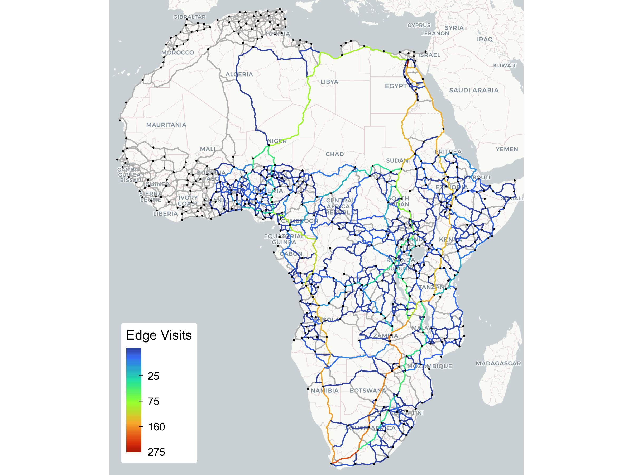
As this plot makes evident, by virtue of the various edge-level statistics run_assignment() can return, it is not necessary to retain the full paths to fully understand the model.
Now, let’s also plot the probabilities. The edge_weights returned by the model represent the sum of path probabilities over all paths using each edge. Thus, in the context of probabilistic assignment, they can be interpreted as the proportion of C2C trade that traverses the edge. For additional clarity, let’s highlight only those edges where the probability is above 0.0001.
africa_net$c2c_eweights[c2c_edges] <- replace_outliers(c2c_eweights, 0.0001, NA, "min")
tm_basemap("CartoDB.Positron", zoom = 4) +
tm_shape(africa_net) +
  tm_lines(col = "c2c_eweights",
           col.scale = tm_scale_continuous_sqrt(6, values = "turbo", limits = c(0, 1),
                                           values.range = c(0.1, 0.9),
                                           value.na = "grey"),
           col.legend = tm_legend("Edge Probabilities", position = c("left", "bottom"),
                                  frame = FALSE, text.size = 0.8, title.size = 1,
                                  item.height = 2, na.show = FALSE), lwd = 1.5) +
tm_shape(africa_cities_ports) + tm_dots(size = 0.1) +
tm_layout(frame = FALSE, outer.margins = 0)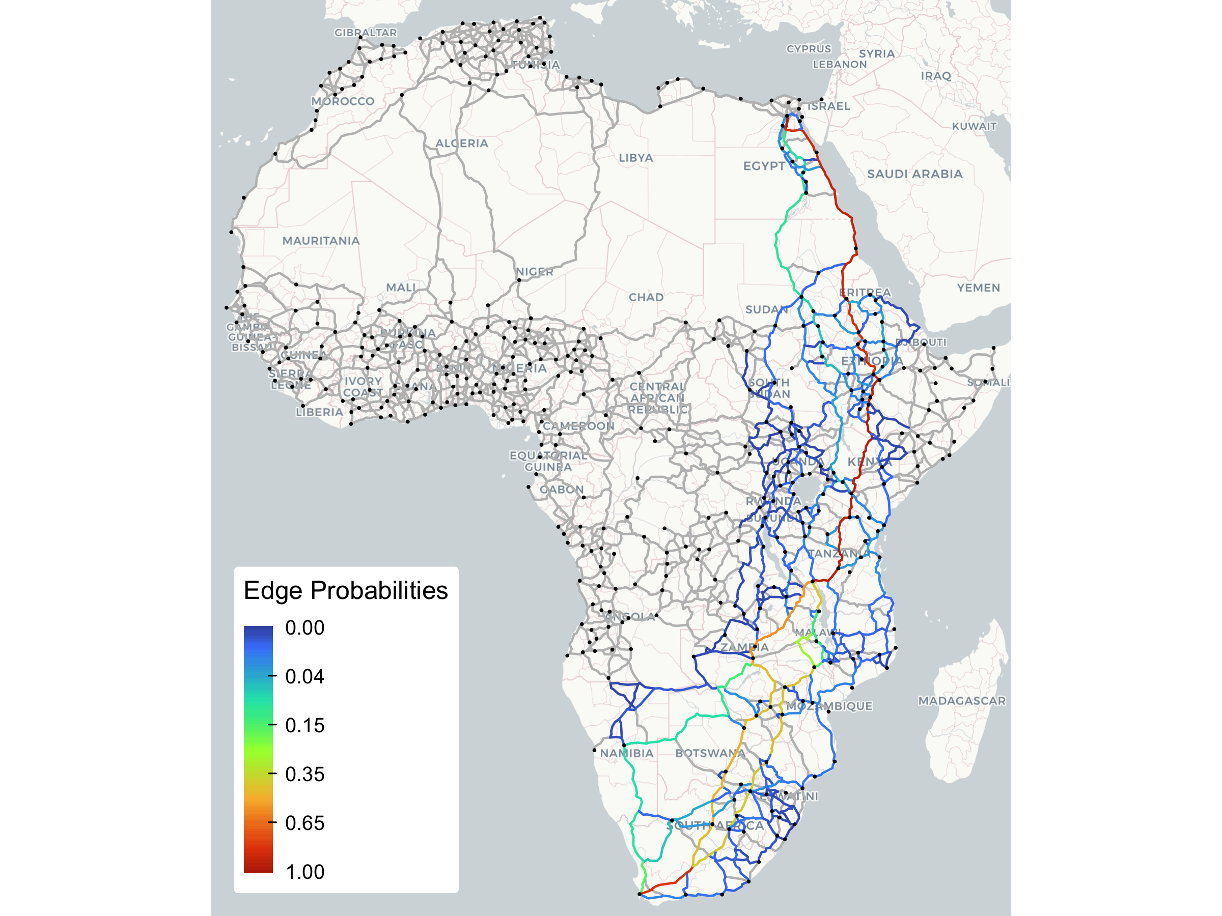
Clearly, and in contrast to what the edge counts from the raw routes suggested, no meaningful C2C traffic is routed through central Africa or the Sahara.
The model thus seems well-behaved, and we can plot the final flows on the entire network:
africa_net$final_flows <- result$final_flows
tm_basemap("CartoDB.Positron", zoom = 4) +
tm_shape(africa_net) +
  tm_lines(col = "final_flows",
           col.scale = tm_scale_continuous_sqrt(values = "turbo",
                                           values.range = c(0.1, 0.9),
                                           value.na = "grey"),
           col.legend = tm_legend("Frictionless Flows", position = c("left", "bottom"),
                                  frame = FALSE, text.size = 0.8, title.size = 1,
                                  item.height = 2, na.show = FALSE), lwd = 1.5) +
tm_shape(africa_cities_ports) + tm_dots(size = 0.1) +
tm_layout(frame = FALSE, outer.margins = 0)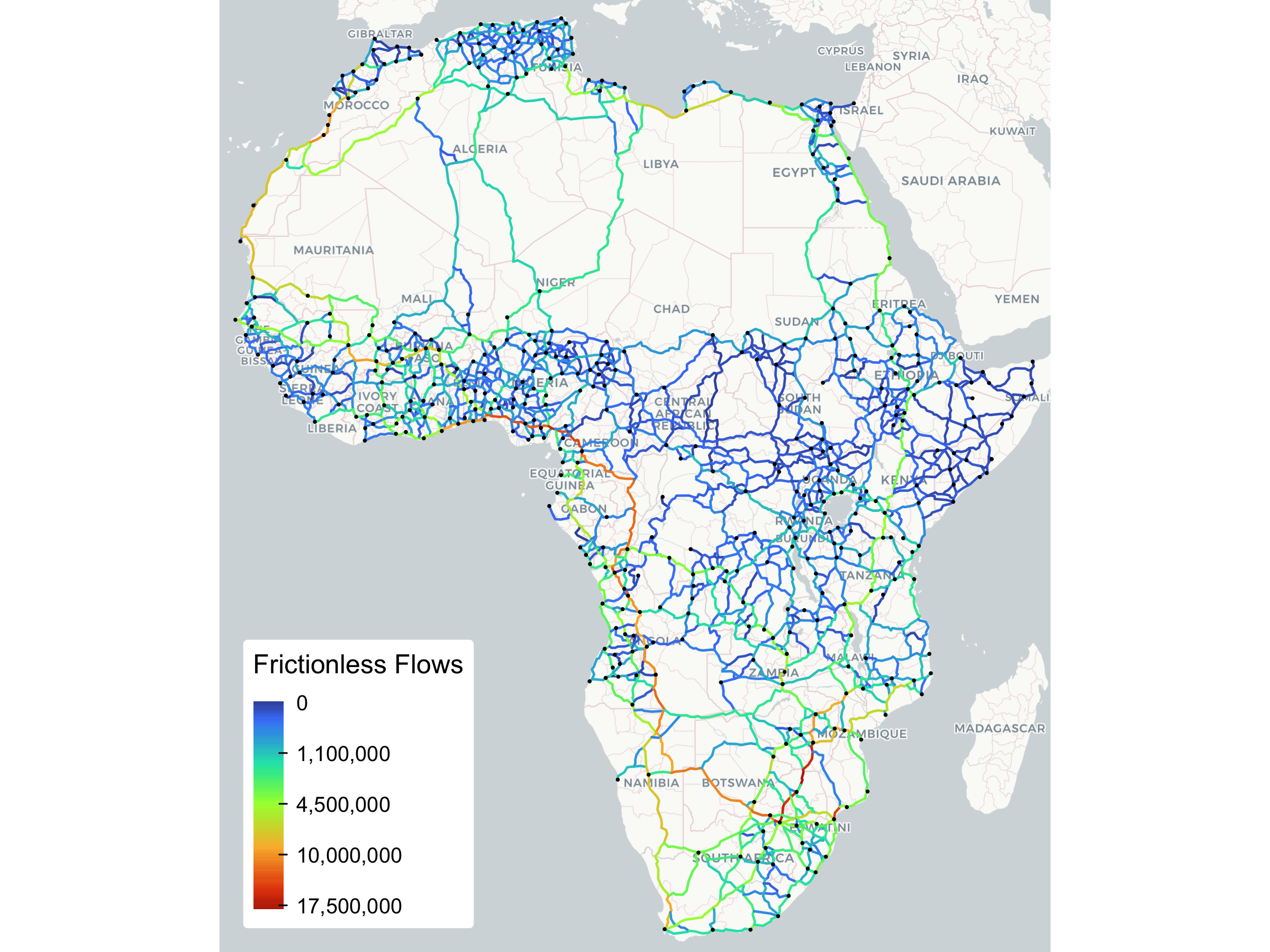
Evidently, certain trade routes are much more utilized than others. But this, of course, assumes the frictionless scenario. Let’s now see how the picture changes with the realistic trade costs added:
# Median scaling cost column: recommended for PSL
settfm(graph, total_time_ms = fmedian(total_time, TRA = "/"))
# Run Traffic Assignment using the PSL model
system.time({
result_tc <- run_assignment(graph, od_matrix_trade, cost.column = "total_time_ms",
                            beta = 4, nthreads = 8, verbose = FALSE)
})
##    user  system elapsed
##  25.675   2.666  27.640
print(result_tc)
## FlowNet object
## Call: run_assignment(graph_df = graph, od_matrix_long = od_matrix_trade,      cost.column = "total_time_ms", beta = 4, verbose = FALSE,      nthreads = 8)
##
## Number of edges: 2344
## Number of simulations/OD-pairs: 189020
##
## Final flows summary statistics:
##      N  Ndist         Mean           SD  Min          Max  Skew   Kurt
##   2344   2314  1'401715.01  3'019114.05    0  32'492559.6  3.86  21.47
##   1%       5%       10%       25%       50%          75%       90%          95%          99%
##    0  3035.57  11555.93  55039.95  273655.4  1'140869.45  3'780896  7'276797.09  16'361834.1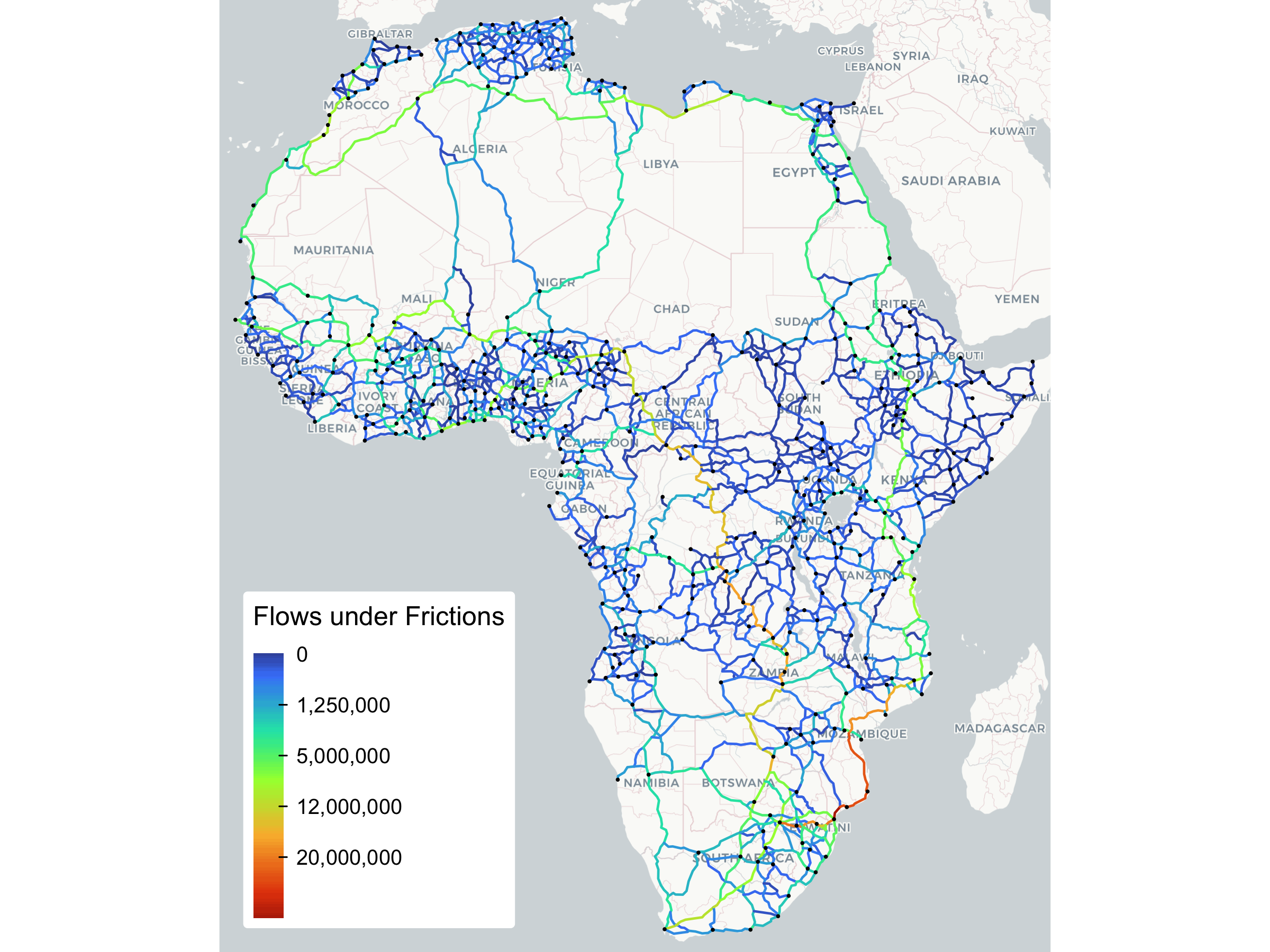
This result is quite fascinating as it suggests that, if the Doing Business 2019 Trade Frictions are accurate and traders are rational, these frictions could strongly distort intra-African trade patterns from the efficient equilibrium determined by the quality of infrastructure. This could be further investigated...
Speaking about infrastructure quality, what if the existing network were fully upgraded? If all roads had a minimum travel speed of 100km/h? The network includes a column duration_100kmh simulating just that. The median link under this scenario has a travel time of only 65% of the current travel time.
quantile(africa_net$duration_100kmh / africa_net$duration, Qprobs)
##         0%         1%         5%        25%        50%        75%        95%        99%       100%
## 0.05142949 0.31306222 0.39842537 0.53691407 0.64688128 0.80874861 0.85202685 0.94515228 1.00000000
settfm(graph, duration_100kmh_ms = fmedian(duration_100kmh, TRA = "/"))
result_ug <- run_assignment(graph, od_matrix_trade, cost.column = "duration_100kmh_ms",
                            beta = 4, nthreads = 8, verbose = FALSE)
print(result_ug)
## FlowNet object
## Call: run_assignment(graph_df = graph, od_matrix_long = od_matrix_trade,      cost.column = "duration_100kmh_ms", beta = 4, verbose = FALSE,      nthreads = 8)
##
## Number of edges: 2344
## Number of simulations/OD-pairs: 189020
##
## Final flows summary statistics:
##      N  Ndist         Mean           SD  Min          Max  Skew   Kurt
##   2344   2312  1'299050.05  2'196434.83    0  15'383521.6  3.45  16.51
##        1%        5%       10%        25%        50%          75%          90%          95%          99%
##   4404.87  27001.59  67602.42  192133.57  537029.72  1'379204.11  3'069293.25  5'558163.65  12'401186.9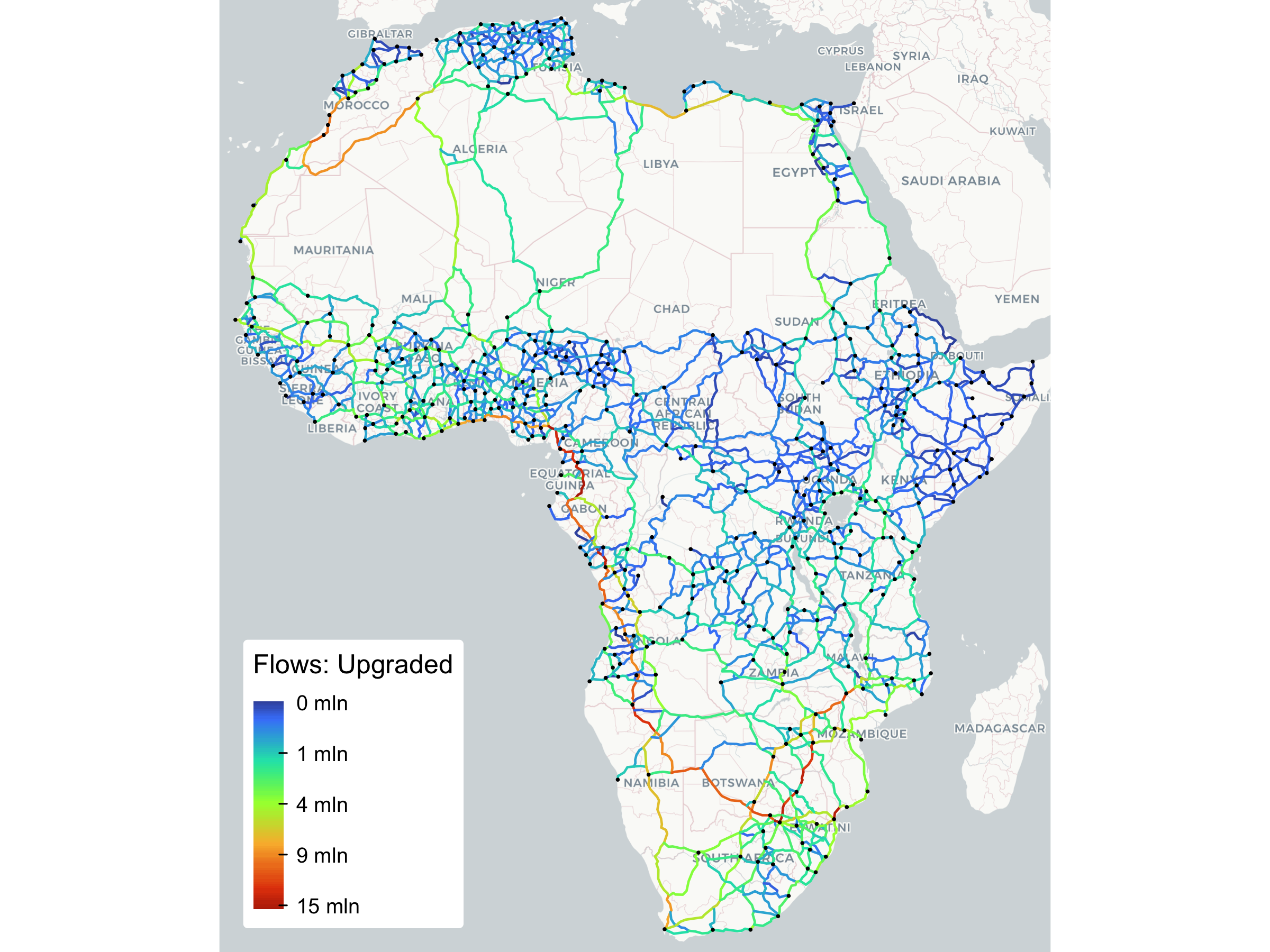
The plot appears similar to the previous frictionless plot, with a bit more traffic routed through central Africa and the Sahara where at present the road quality is very poor. However, given the present low volume of trade between Eastern and Western Africa (less than 1% of total intra-African trade), paving roads in central Africa wouldn’t pay off. Such investments thus appear hinged on changing regional trade patterns, and, as the paper finds using a generative gravity-like spatial equilibrium model that does allow trade flows to adjust to infrastructure changes, on unrealistically low trade elasticities.
Lastly, we can simulate flows on the network with the proposed links added, and see how much they would be utilized. These links, although drawn as straight lines, are assumed to be 1.2 times longer than the line, which is the average across existing links when comparing them to a straight line.
qDT(africa_network)[add == TRUE, quantile(distance / sp_distance)]
##      0%     25%     50%     75%    100%
## 1.20812 1.20812 1.20812 1.20812 1.20812
They are given a speed of 100km/h, and I will also assume the existing network was upgraded first.
graph_total <- st_drop_geometry(africa_network)
settfm(graph_total, duration_100kmh_ms = fmedian(duration_100kmh, TRA = "/"))
result_add <- run_assignment(graph_total, od_matrix_trade,
                             cost.column = "duration_100kmh_ms",
                             beta = 4, nthreads = 8, verbose = FALSE)
print(result_add)
## FlowNet object
## Call: run_assignment(graph_df = graph_total, od_matrix_long = od_matrix_trade,      cost.column = "duration_100kmh_ms", beta = 4, verbose = FALSE,      nthreads = 8)
##
## Number of edges: 2825
## Number of simulations/OD-pairs: 189020
##
## Final flows summary statistics:
##      N  Ndist       Mean           SD  Min          Max  Skew  Kurt
##   2825   2789  943826.09  1'718125.92    0  16'443663.3  4.22  25.5
##   1%        5%       10%        25%        50%     75%          90%         95%          99%
##    0  14333.81  34879.15  121091.46  361495.66  980800  2'313254.89  3'765464.8  9'265394.48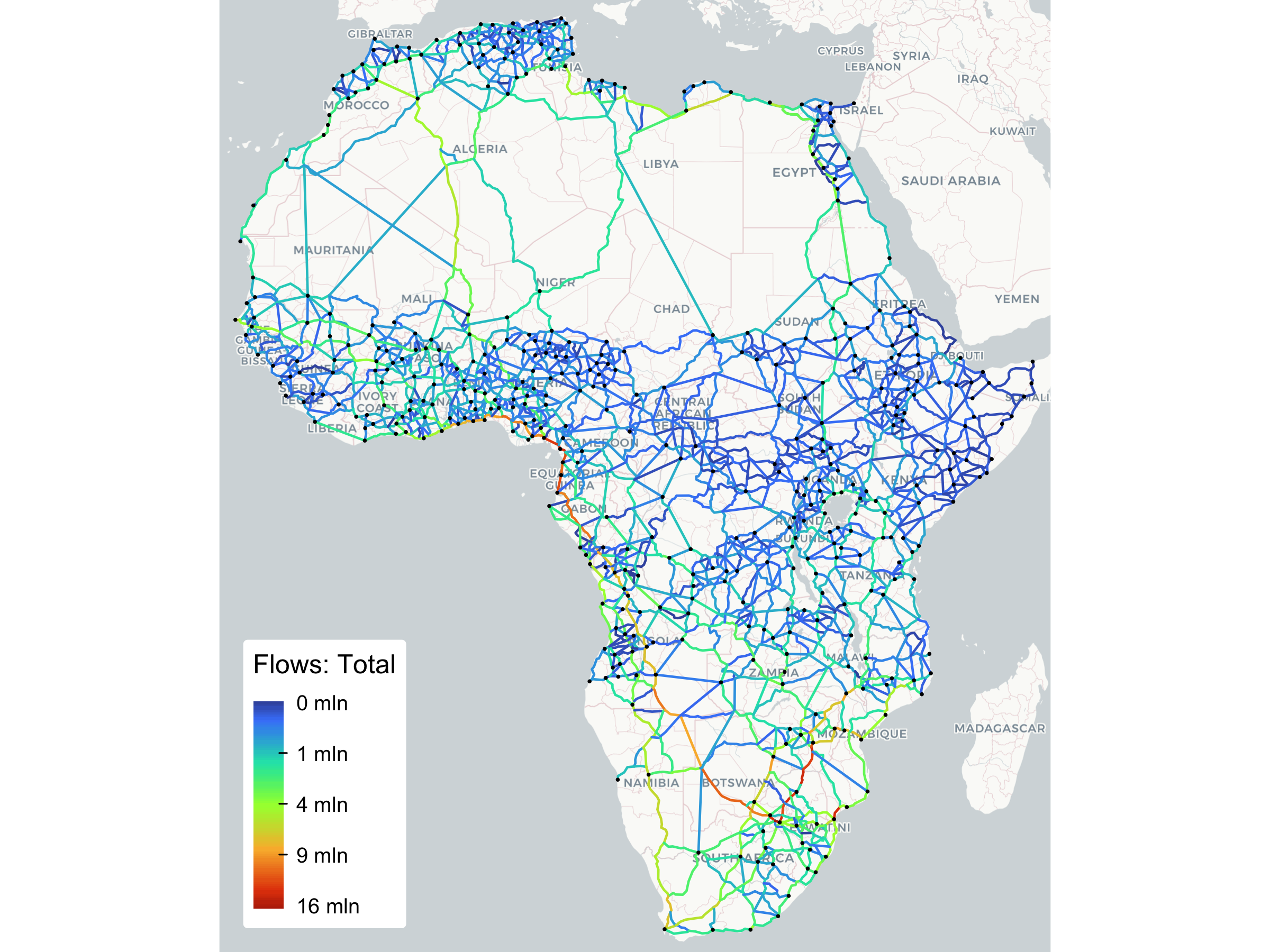
The results suggest that some new national links, e.g., in Botswana, additional trans-Saharan links, and reopening the Morocco-Algeria border, could be utilized significantly under current trade patterns.
Let me note again that all of this assumes intra-African trade patterns are static, which of course they are not, as infrastructure improvements can alter trade flows. The joint endogeneity of infrastructure and trade is appropriately handled in the paper, building on Fajgelbaum and Schaal (2020).
Example 2: The US Freight Analysis Framework (FAF) Network
The Freight Analysis Framework (FAF), produced jointly by the Bureau of Transportation Statistics (BTS) and the Federal Highway Administration (FHWA), integrates data from a variety of sources—most notably the Commodity Flow Survey—to create a comprehensive picture of freight movement among US states and major metropolitan areas by all modes of transportation. It provides estimates of tonnage, value, and domestic ton-miles by origin-destination pairs, commodity type, and transportation mode, along with 30-year forecasts through 2050 under different economic growth scenarios.
The latest version, FAF5, is benchmarked on the 2017 Commodity Flow Survey and includes a model highway network with 487,384 links and 348,498 nodes. The links cover all roads in the National Highway System (NHS) and the National Highway Freight Network (NHFN) that are currently open to traffic. FAF5 also provides truck flow assignments that route commodity movements onto this highway network. An update to FAF6, benchmarked on the 2022 Commodity Flow Survey, is expected in 2026.
We begin by loading the network links from a geodatabase using st_read().
# Loading FAF5 network from geodatabase format
FAF5 <- st_read(FAF5_path, layer = "FAF5_Links")
## Reading layer `FAF5_Links' from data source `/Users/sebastiankrantz/Documents/CPCS/FAF5/Networks/Geodatabase Format/FAF5Network.gdb' using driver `OpenFileGDB'
## Simple feature collection with 487394 features and 52 fields
## Geometry type: MULTILINESTRING
## Dimension:     XY
## Bounding box:  xmin: -167.0152 ymin: 18.91474 xmax: -66.98005 ymax: 71.3198
## Geodetic CRS:  NAD83
nrow(FAF5)
## [1] 487394
table(vlengths(FAF5$SHAPE))
##
##      1
## 487394
head(FAF5, 1)
## Simple feature collection with 1 feature and 52 fields
## Geometry type: MULTILINESTRING
## Dimension:     XY
## Bounding box:  xmin: -132.9754 ymin: 56.80636 xmax: -132.975 ymax: 56.80701
## Geodetic CRS:  NAD83
##   ID     LENGTH DIR    DATA  VERSION Class               Class_Description                    Road_Name Sign_Rte Rte_Type Rte_Number Rte_Qualifier
## 1  1 0.05408278   1 1324805 V2021.05    19 Facility Access/Circulator Road PETERSBURG FERRY TERMINAL RD     <NA>     <NA>       <NA>          <NA>
##   Country STATE STFIPS County_Name CTFIPS Urban_Code FAFZONE Status F_Class Facility_Type NHS STRAHNET NHFN Truck AB_Lanes BA_Lanes Speed_Limit
## 1     USA    AK     02  PETERSBURG  02195      99999      20      1       5            NA  NA       NA   NA  <NA>        1       NA          10
##   Toll_Type Toll_Name Toll_Link Toll_Link_Name HPMS_USA_RouteID HPMS_Begin_Point HPMS_End_Point BorderState1 BorderState2 BorderFAF1 BorderFAF2
## 1        NA      <NA>        NA           <NA>             <NA>               NA             NA         <NA>         <NA>         NA         NA
##   TRUCKTOLL BorderLink AddedBorderTime AdjustSpeed AdjustReason AB_FinalSpeed BA_FinalSpeed AB_CombinedSpeed BA_CombinedSpeed AB_FreeFlowTime
## 1        NA         NA              NA          NA         <NA>            43            43               43               43      0.07546435
##   BA_FreeFlowTime SHAPE_Length                          SHAPE
## 1      0.07546435  0.001008685 MULTILINESTRING ((-132.975 ...
The FAF5 network is large and spatially accurate—too large to visualize in R—but you can view it online.
The SHAPE column contains MULTILINESTRING geometries, but, as table(vlengths(FAF5$SHAPE)) confirms, all are of length 1 and can be cast to simple LINESTRINGs. This is required by flownet::linestrings_to_graph(), which matches start and end points across linestrings to build a graph, subject to a numerical tolerance (by default, 6-digit rounding \(\approx\) 11cm at the equator). To ensure this rounding is properly applied, we also transform the coordinates to WGS84 (EPSG:4326).
graph <- FAF5 |> st_cast("LINESTRING") |> st_transform(4326) |>
    linestrings_to_graph()
nrow(graph)
## [1] 487394
graph[1:5, 1:10]
##   edge from        FX       FY to        TX       TY         .length ID      LENGTH
## 1    1    1 -132.9750 56.80636  2 -132.9750 56.80701    86.86074 [m]  1  0.05408278
## 2    2    2 -132.9750 56.80701  4 -132.9762 56.80849   184.49595 [m]  2  0.11485356
## 3    3    2 -132.9750 56.80701  3 -132.9746 56.80664    52.08027 [m]  3  0.03243200
## 4    4    3 -132.9746 56.80664  6 -132.9601 56.80941  1004.86210 [m]  4  0.62628710
## 5    5    4 -132.9762 56.80849 10 -132.6638 56.71238 24432.32444 [m]  5 15.22300434
# 'edge' is always unique
any_duplicated(graph$edge)
## [1] FALSE
# But there may be duplicate edges between the same from-to nodes
sum(fduplicated(graph[, c("from", "to")]))
## [1] 679
Evidently, casting to LINESTRING did not increase the row count in this case. linestrings_to_graph() then removed the geometry (SHAPE) column and added 8 columns: a unique edge identifier, from and to node IDs with corresponding geodetic coordinates (WGS84), and .length computed directly from the shape in meters (which here matches the LENGTH column expressed in miles).
We can again extract nodes with nodes_from_graph() to determine the nearest node to each of the 3796 FAF5 zones provided as origin and destination locations for commodity flows:
zones <- st_read(FAF5_path, layer = "FAF5_Nodes") |>
  fsubset(!is.na(CentroidID)) |> st_transform(4326)
## Reading layer `FAF5_Nodes' from data source `/Users/sebastiankrantz/Documents/CPCS/FAF5/Networks/Geodatabase Format/FAF5Network.gdb' using driver `OpenFileGDB'
## Simple feature collection with 974788 features and 15 fields
## Geometry type: POINT
## Dimension:     XY
## Bounding box:  xmin: -167.0152 ymin: 18.91474 xmax: -66.98005 ymax: 71.3198
## Geodetic CRS:  NAD83
nrow(zones)
## [1] 3796
head(zones, 1)
## Simple feature collection with 1 feature and 15 fields
## Geometry type: POINT
## Dimension:     XY
## Bounding box:  xmin: -132.9393 ymin: 56.83877 xmax: -132.9393 ymax: 56.83877
## Geodetic CRS:  WGS 84
##   ID     DATA Entry_or_Exit Exit_Number Interchange Centroid CentroidID Facility_Type Facility_Name County State StateID StateName FAFID StateNameBak
## 1 14 47179393          <NA>        <NA>        <NA>        1       2195          <NA>          <NA>   <NA>  <NA>       2    Alaska    20       Alaska
##                        SHAPE
## 1 POINT (-132.9393 56.83877)
nodes <- nodes_from_graph(graph, sf = TRUE)
nrow(nodes)
## [1] 348495
Using the FAF5 Data Tabulation Tool, I have generated an OD matrix of total 2024 truck flows:
OD <- fread(FAF5_2024_truck_flows) |> janitor::clean_names() |>
  ftransform(id_o = as.integer(substr(dms_orig, 1, 3)),
             id_d = as.integer(substr(dms_dest, 1, 3)))
nrow(OD)
## [1] 16798
head(OD, 3)
##             dms_orig          dms_dest dms_mode thousand_tons_in_2024  id_o  id_d
##               <char>            <char>   <char>                 <num> <int> <int>
## 1: 011-Birmingham AL 011-Birmingham AL  1-Truck            35382.9943    11    11
## 2: 011-Birmingham AL     012-Mobile AL  1-Truck              970.8396    11    12
## 3: 011-Birmingham AL    019-Rest of AL  1-Truck            10178.2525    11    19
This data can be matched to zone nodes, but only at the coarser 3-digit FAF zone level:
zones |> join(fslice(OD, id_o), on = c("FAFID" = "id_o")) |> invisible()
## left join: zones[FAFID] 3796/3796 (100%) <28.76:1st> y[id_o] 132/132 (100%)
zones |> join(fslice(OD, id_d), on = c("FAFID" = "id_d")) |> invisible()
## left join: zones[FAFID] 3796/3796 (100%) <28.76:1st> y[id_d] 132/132 (100%)
We therefore aggregate the centroids to the 3-digit level and map them to the nearest network nodes:
# Aggregating zones and computing aggregate centroids
zones_agg <- zones |> fgroup_by(FAFID) |>
  fsummarise(SHAPE = st_centroid(st_combine(SHAPE)))
# Matching each aggregate zone centroid to the nearest network node
zones_agg$NN <- nodes$node[st_nearest_feature(zones_agg, nodes)]
We are now ready to create a mapped OD-matrix with from and to node columns as well as flow:
OD_mapped <- OD |>
  join(zones_agg |> st_drop_geometry() |> fselect(FAFID, NN),
       on = c("id_o" = "FAFID")) |> frename(from = NN) |>
  join(zones_agg |> st_drop_geometry() |> fselect(FAFID, NN),
       on = c("id_d" = "FAFID")) |> frename(to = NN) |>
  fmutate(flow = thousand_tons_in_2024) |>
  fsubset(is.finite(flow) / flow > 0, from, dms_orig, to, dms_dest, flow)
## left join: OD[id_o] 16798/16798 (100%) <127.26:1st> y[FAFID] 132/132 (100%)
## left join: x[id_d] 16798/16798 (100%) <127.26:1st> y[FAFID] 132/132 (100%)
head(OD_mapped)
##     from          dms_orig     to          dms_dest       flow
##    <int>            <char>  <int>            <char>      <num>
## 1:  6551 011-Birmingham AL   6551 011-Birmingham AL 35382.9943
## 2:  6551 011-Birmingham AL 124499     012-Mobile AL   970.8396
## 3:  6551 011-Birmingham AL 125253    019-Rest of AL 10178.2525
## 4:  6551 011-Birmingham AL   1691        020-Alaska     0.0000
## 5:  6551 011-Birmingham AL  15659    041-Phoenix AZ    50.0572
## 6:  6551 011-Birmingham AL   5981     042-Tucson AZ     1.3969
Let us now proceed to a basic flows assignment using the efficient All-or-Nothing (AoN) method. Before running it, we need to further process the graph in two ways:
- Create a column representing the generalized cost of traversing a link.
- Ensure directed links are properly represented.
For (1), I combine the free flow time (in minutes) with a truck toll estimate (average per-mile toll for a 5-axle vehicle \(\times\) segment length), converted to minutes assuming a value of time (VOT) of 50 USD/hour.
fnobs(graph$TRUCKTOLL) # Number of links with tolls
## [1] 3245
graph %<>% fmutate(TollTime = replace_na(TRUCKTOLL, 0) / 50 * 60,
                   cost_AB = replace_na(AB_FreeFlowTime + TollTime, 1e4),
                   cost_BA = replace_na(BA_FreeFlowTime + TollTime, 1e4))
graph %$% fquantile(setv(TollTime / cost_AB, 0, NA), Qprobs)
##         0%         1%         5%        25%        50%        75%        95%        99%       100%
## 0.09420283 0.11402505 0.13810940 0.22898990 0.28057551 0.84988865 0.98935454 0.99612581 0.99964115
Among the 3245 links with tolls, tolls account for ~28% of the generalized cost. A few links (~3800 in each direction) are missing free flow time; these are imputed with a very high cost of 10,000 minutes.
The network provides free flow time estimates in both directions, and, to complicate things further, a DIR column indicates whether the link is bidirectional (0) or unidirectional (1 or -1). We thus need to convert the graph to a fully directed one by duplicating bidirectional links with swapped endpoints.
table(graph$DIR) # See direction or undirectedness of links
##
##     -1      0      1
##    391 168215 318788
# Create fully directed graph representation
graph_dir <- rowbind(
   graph |> fselect(from, to, FX, FY, TX, TY, cost = cost_AB),
   graph |> fsubset(DIR == 0,
     from = to, to = from, FX = TX, FY = TY, TX = FX, TY = FY, cost = cost_BA)
)
nrow(graph_dir)
## [1] 655609
We are now ready for directed All-or-Nothing assignment:
system.time({
result_AoN <- run_assignment(graph_dir, OD_mapped, directed = TRUE,
     method = "AoN", return.extra = "costs", verbose = FALSE)
})
##    user  system elapsed
##  10.310   0.199  10.519
print(result_AoN)
## FlowNet object
## Call: run_assignment(graph_df = graph_dir, od_matrix_long = OD_mapped,      directed = TRUE, method = "AoN", return.extra = "costs",      verbose = FALSE)
##
## Number of edges: 655609
## Number of simulations/OD-pairs: 16438
##
## Average path cost (SD): 1207.033  (759.4758)
##
## Final flows summary statistics:
##        N  Ndist     Mean       SD  Min        Max  Skew   Kurt
##   655609   5401  1948.29  6721.89    0  137376.81  4.99  35.61
##   1%  5%  10%  25%  50%  75%      90%       95%       99%
##    0   0    0    0    0    0  5378.46  15025.71  34257.51
The igraph library called under the hood still warns about some unreachable nodes, leaving 16798-16438 = 360 OD-pairs unassigned. A remedy would be to duplicate all directed links with a very high cost in the opposite direction, but with 655,609 edges already, further edge inflation is undesirable.
As noted above, this network is a borderline case for PSL assignment in terms of computational complexity, but, with only ~16.8k OD-pairs, we can manage by restricting detours to 1.2\(\times\) the shortest path and the angle for intermediate target nodes to 30 degrees.2 Since the US network is very route efficient, these restrictions are reasonable. They do not fully tame the combinatorial explosion, however—some connections (e.g., San Francisco to New York) still admit over 90,000 alternatives—so we additionally cap the number of paths at a random sample of 1000.3 For memory-efficient multithreading, I also limit the pre-computed OD cost and geodesic distance matrices to 5000\(^2\).
We also need to calibrate the PSL model. The average path cost here is 1207 minutes—exponentiating such large numbers in the MNL concentrates virtually all probability on the shortest path, reducing the PSL to AoN. Having calibrated the Africa model with beta = 4 at an average normalized cost of 53.5, I apply a heuristic scaling of 53.5 / 1207 = 0.0443 to the FAF5 link costs and reuse the same beta.
graph_dir$cost_scaled <- graph_dir$cost * 53.5 / 1207
system.time({
result_PSL <- run_assignment(
    graph_dir, OD_mapped, directed = TRUE,
    cost.column = "cost_scaled", method = "PSL", beta = 4,
    detour.max = 1.2, angle.max = 30, npaths.max = 1000,
    dmat.max.size = 5000^2, nthreads = 8, verbose = FALSE,
    return.extra = c("edges", "counts", "weights", "eweights")
) |> suppressWarnings()
})
##    user  system elapsed
## 444.772  20.004 476.424
print(result_PSL)
## FlowNet object
## Call: run_assignment(graph_df = graph_dir, od_matrix_long = OD_mapped,      directed = TRUE, cost.column = "cost_scaled", method = "PSL",      beta = 4, detour.max = 1.2, angle.max = 30, npaths.max = 1000,      dmat.max.size = 5000^2, return.extra = c("edges", "counts",          "weights", "eweights"), verbose = FALSE, nthreads = 8)
##
## Number of edges: 655609
## Number of simulations/OD-pairs: 16438
##
## Average number of edges utilized per simulation (SD): 13803.19  (8072.216)
## Average number of visits per edge (SD): 28.39304  (69.88708)
## Average path weight (SD): 0.002916186  (0.01594657)
## Average summed edge weight (SD): 0.06338159  (0.18493)
##
## Final flows summary statistics:
##        N   Ndist     Mean       SD  Min        Max  Skew   Kurt
##   655609  397919  1882.31  5631.94    0  132405.13  4.86  35.47
##   1%  5%  10%   25%    50%     75%      90%       95%       99%
##    0   0    0  0.79  25.25  464.02  5373.66  12819.44  28378.51
Solving 16,438 OD pairs (\(\leq\) 1000 paths each) in about 8 minutes—again generating around 15 million paths, but on a network with 253\(\times\) more nodes and 280\(\times\) more edges than the Africa network, while taking only 16\(\times\) more time—is rather impressive. Still, the throughput of only ~35 OD pairs per second imposes clear limits for considering much larger OD matrices.4
Now that we have a result, let’s visualize the generated routes from San Francisco to New York.
sf2ny <- OD_mapped |>
  with(which(dms_orig %like% "San Francisco" & dms_dest %like% "363-New York"))
# Here we need to adjust the index because some OD pairs were removed
sf2ny <- whichv(result_PSL$od_pairs_used, sf2ny)
length(result_PSL$path_weights[[sf2ny]]) # Number of paths retained
## [1] 408
sf2ny_edges <- result_PSL$edges[[sf2ny]]
sf2ny_net <- linestrings_from_graph(ss(graph_dir, sf2ny_edges))
sf2ny_net$edge_counts <- result_PSL$edge_counts[[sf2ny]]
sf2ny_net$edge_weights <- result_PSL$edge_weights[[sf2ny]]

tm_basemap("CartoDB.Positron", zoom = 4) +
tm_shape(roworder(sf2ny_net, edge_counts)) +
  tm_lines(col = "edge_counts",
           col.scale = tm_scale_continuous_sqrt(6, values = "turbo",
                                           values.range = c(0.1, 0.9),
                                           value.na = "grey"),
           col.legend = tm_legend("Edge Visits", position = c("left", "bottom"),
                                  orientation = "landscape",
                                  frame = FALSE, text.size = 0.8, title.size = 1,
                                  item.width = 3, bg.alpha = 0.6,
                                  na.show = FALSE), lwd = 1.5) +
tm_shape(zones_agg) + tm_dots(size = 0.1) +
tm_layout(frame = FALSE, outer.margins = 0)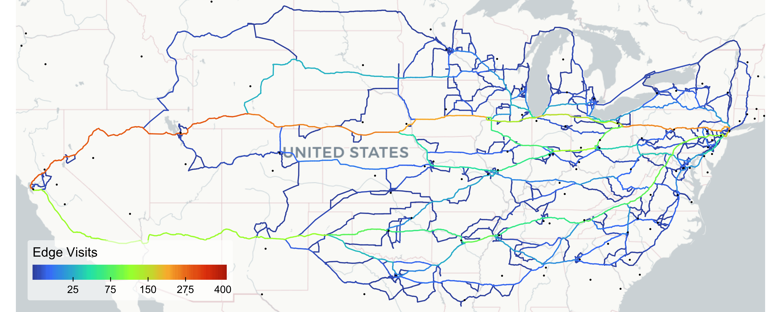
As expected, we obtain a large number of paths, many of which take curious detours. The route enumeration algorithm filters out paths with duplicate directional edges, ensuring no route traverses a road segment twice—this ex-post elimination is the main reason we retain only 408 of the sampled 1000. Some intermediate nodes generating valid routes lie inside city centers or in the open field, yielding complex local patterns. Nonetheless, the edge counts clearly reveal two main corridors (north and south), both branching out as they approach New York.
Let’s now see what the edge probabilities suggest where traffic is actually going:
# Again clipping small probabilities below 0.0001
sf2ny_net$edge_weights_clip <- replace_outliers(sf2ny_net$edge_weights, 0.0001, NA, "min")
tm_basemap("CartoDB.Positron", zoom = 4) +
tm_shape(roworder(sf2ny_net, edge_weights_clip)) +
  tm_lines(col = "edge_weights_clip",
           col.scale = tm_scale_continuous_sqrt(6, values = "turbo", limits = c(0, 1),
                                           values.range = c(0.1, 0.9),
                                           value.na = "grey"),
           col.legend = tm_legend("Edge Probabilities", position = c("left", "bottom"),
                                  orientation = "landscape",
                                  frame = FALSE, text.size = 0.8, title.size = 1,
                                  item.width = 3, bg.alpha = 0.6,
                                  na.show = FALSE), lwd = 1.5) +
tm_shape(zones_agg) + tm_dots(size = 0.1) +
tm_layout(frame = FALSE, outer.margins = 0)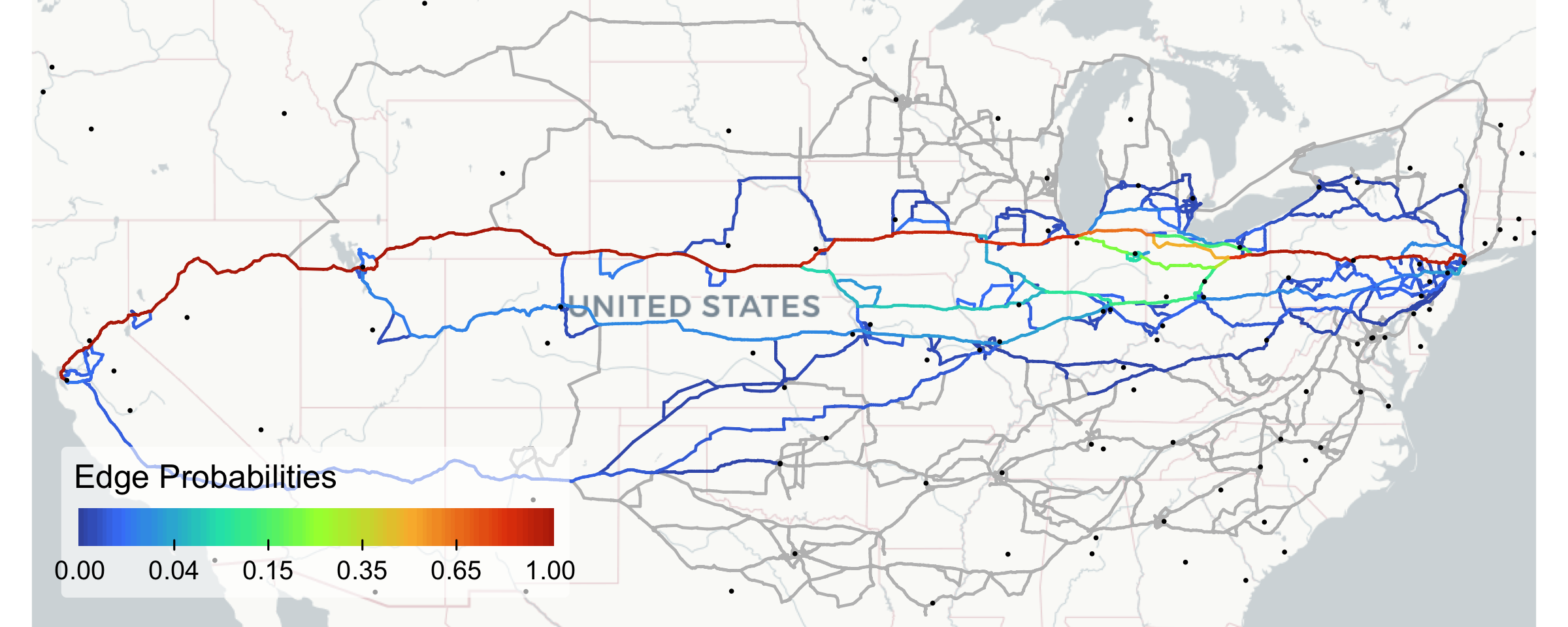
The southern route is clearly not deemed very viable by the MNL function. Most traffic follows the northern corridor, with meaningful heterogeneity only in the Midwest where it splits into a few near-equally probable branches that later merge. A minor southern variant carries about 5% of traffic.
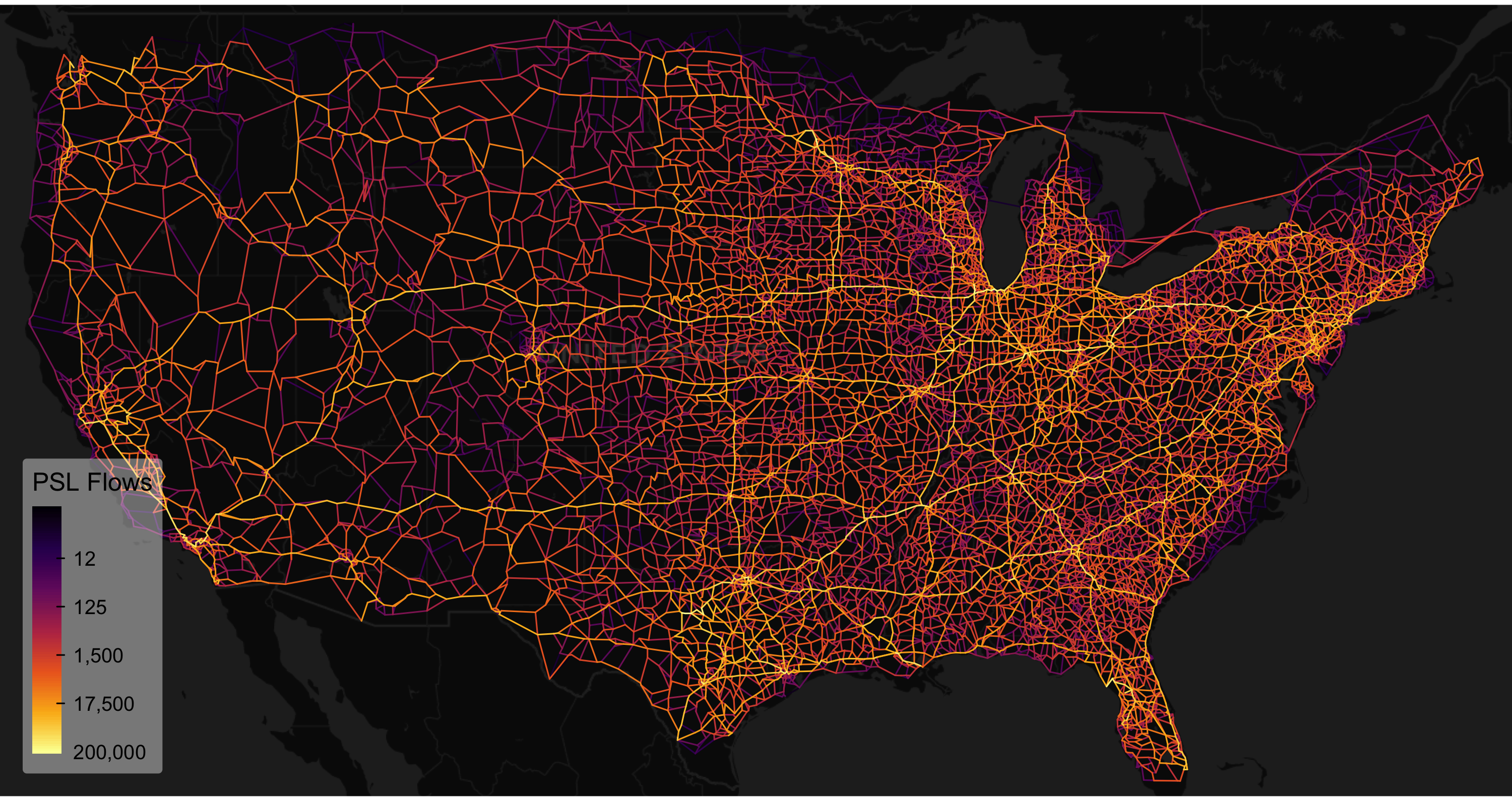
As with the Africa network, the PSL model imposes economically sound structure on a large set of heterogeneous routes. Let us now attempt to visualize the full network flows. To reduce spatial complexity, we will aggregate the directed graph back to an undirected one and filter out links with negligible flows, as well as links going to Alaska (upwards of 49.1 degrees latitude).
flows <- graph_dir %>%
  ftransform(flows = result_PSL$final_flows,
             from = fpmax(from, to), to = fpmin(from, to)) %>%
  fgroup_by(from, to) %>%
  fsummarise(across(FX:TY, ffirst),
             flows = fsum(flows),
             cost = fmean(cost)) %>%
  fsubset(flows > 1 & FY < 49.1 & TY < 49.1)
head(flows, 3)
##   from to        FX       FY        TX       TY     flows      cost
## 1   94 93 -117.7272 33.48681 -117.7854 33.54277  1184.096 8.0597573
## 2   95 94 -117.7272 33.48681 -117.7067 33.46553  1184.096 3.0502339
## 3  100 99 -117.4452 33.27583 -117.4406 33.27092 13576.867 0.4469114
For the visualization, I use a dark map and order links by flow so the important ones are plotted last.5
tm_basemap("CartoDB.DarkMatter", zoom = 4) +
tm_shape(roworder(linestrings_from_graph(flows), flows)) +
  tm_lines(col = "flows",
           col.scale = tm_scale_continuous_log(6, values = "inferno"),
           col.legend = tm_legend("PSL Flows", position = c("left", "bottom"),
                                  frame = FALSE, text.size = 0.8, title.size = 1,
                                  item.height = 2, na.show = FALSE, bg.alpha = 0.4), lwd = 0.5) +
tm_layout(frame = FALSE, outer.margins = 0)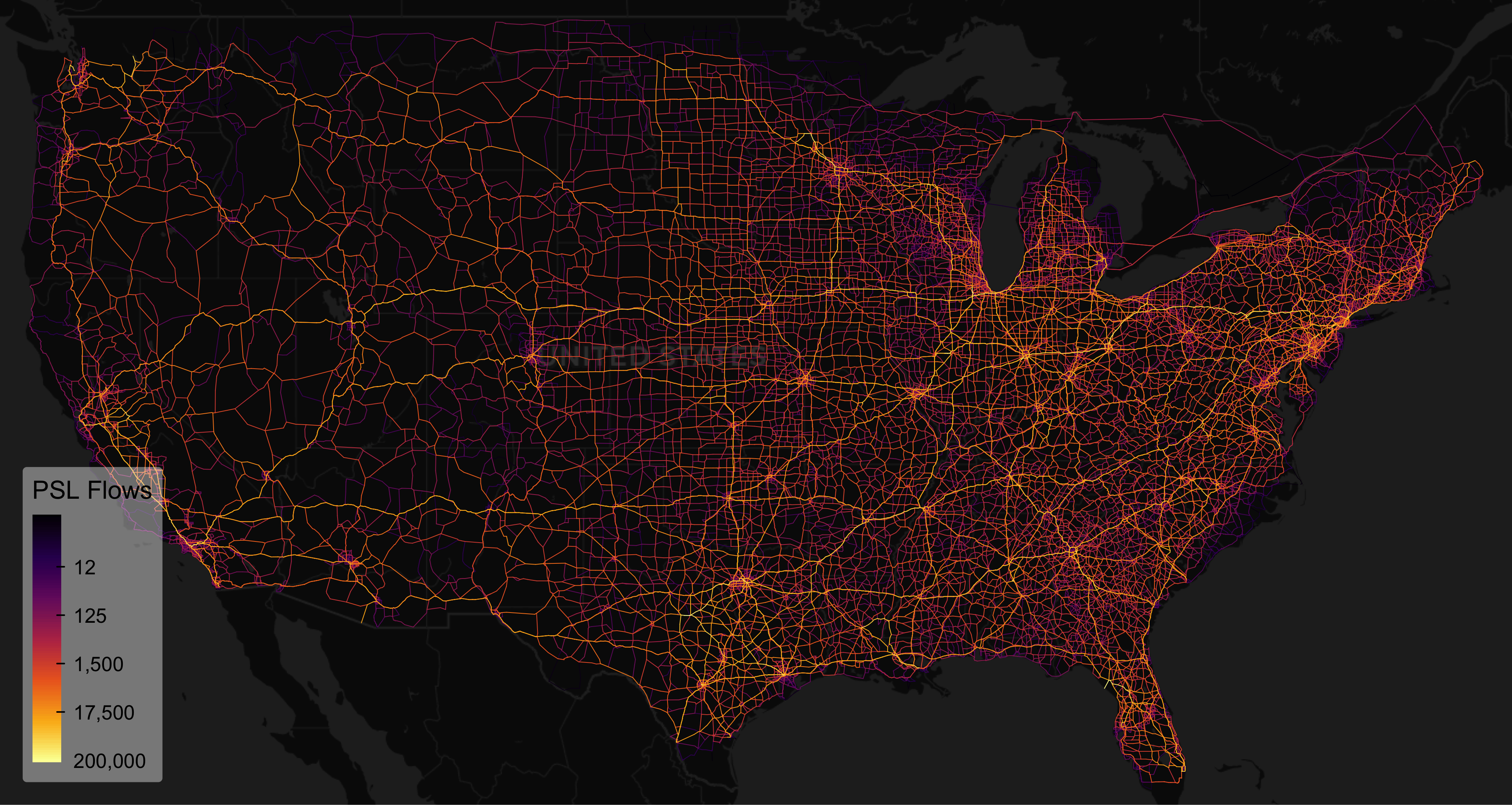
To speed up PSL assignments on very large networks, permitting the use of larger OD matrices within reasonable computing times, we can also use several graph simplification tools flownet provides.
The first, consolidate_graph(), reduces graph complexity by contracting intermediate nodes that connect only two edges, and dropping singleton, loop, and duplicate edges. It supports several levels of recursion: recursive = "full" (the default) repeats edge elimination, node contraction, and attribute aggregation until convergence, yielding the most compact result but making it impossible to trace it back to the original edges. recursive = "partial" omits the aggregation step from the recursion loop and attaches attributes mapping to original edges. This is useful particularly when a more detailed network geometry needs to be unionized along with the graph consolidation for visualization purposes. For aggregation, consolidate_graph() delegates to collap() in collapse, which supports multi-type and custom aggregation with different functions and weights.6 Below, I apply full recursive consolidation on this directed graph, summing all numeric columns (here only "cost" is aggregated).
graph_dir_c <- consolidate_graph(graph_dir, keep = zones_agg$NN, directed = TRUE, FUN = "fsum")
## Consolidating directed graph graph_dir with 655609 edges using full recursion
## Initial node degrees:
##      1      2      3      4      5      6      7      8      9     10     11     12
##  12478  50928 135599  53020  26793  56446   1257  11574     40    351      3      6
##
## Dropped 47 loop edges
## Dropped 1090 duplicate edges
## Dropped 12358 edges leading to singleton nodes
## Dropped 2164 edges leading to singleton nodes
## Dropped 43 edges leading to singleton nodes
## Dropped 9 edges leading to singleton nodes
## Dropped 4 edges leading to singleton nodes
## Dropped 1 edges leading to singleton nodes
## Contracted 61403 intermediate nodes
## Dropped 12 edges leading to singleton nodes
## Aggregated 639881 edges down to 578232 edges
## Dropped 4872 loop edges
## Dropped 5 edges leading to singleton nodes
## Dropped 1 edges leading to singleton nodes
## Contracted 1031 intermediate nodes
## Dropped 10 edges leading to singleton nodes
## Aggregated 573344 edges down to 572279 edges
## Dropped 598 loop edges
## Contracted 287 intermediate nodes
## Dropped 2 edges leading to singleton nodes
## Aggregated 571679 edges down to 571384 edges
## Dropped 227 loop edges
## Contracted 122 intermediate nodes
## Aggregated 571157 edges down to 571030 edges
## Dropped 109 loop edges
## Contracted 58 intermediate nodes
## Aggregated 570921 edges down to 570862 edges
## Dropped 52 loop edges
## Contracted 36 intermediate nodes
## Aggregated 570810 edges down to 570774 edges
## Dropped 33 loop edges
## Contracted 27 intermediate nodes
## Aggregated 570741 edges down to 570714 edges
## Dropped 27 loop edges
## Contracted 23 intermediate nodes
## Aggregated 570687 edges down to 570663 edges
## Dropped 22 loop edges
## Contracted 15 intermediate nodes
## Aggregated 570641 edges down to 570626 edges
## Dropped 15 loop edges
## Contracted 13 intermediate nodes
## Aggregated 570611 edges down to 570598 edges
## Dropped 13 loop edges
## Contracted 11 intermediate nodes
## Aggregated 570585 edges down to 570574 edges
## Dropped 11 loop edges
## Contracted 10 intermediate nodes
## Aggregated 570563 edges down to 570553 edges
## Dropped 10 loop edges
## Contracted 7 intermediate nodes
## Aggregated 570543 edges down to 570536 edges
## Dropped 7 loop edges
## Contracted 4 intermediate nodes
## Aggregated 570529 edges down to 570525 edges
## Dropped 4 loop edges
## Contracted 4 intermediate nodes
## Aggregated 570521 edges down to 570517 edges
## Dropped 4 loop edges
## Contracted 2 intermediate nodes
## Aggregated 570513 edges down to 570511 edges
## Dropped 2 loop edges
## Contracted 2 intermediate nodes
## Aggregated 570509 edges down to 570507 edges
## Dropped 2 loop edges
## Contracted 2 intermediate nodes
## Aggregated 570505 edges down to 570503 edges
## Dropped 2 loop edges
## Contracted 2 intermediate nodes
## Aggregated 570501 edges down to 570499 edges
## Dropped 2 loop edges
## Contracted 2 intermediate nodes
## Aggregated 570497 edges down to 570495 edges
## Dropped 2 loop edges
## Contracted 2 intermediate nodes
## Aggregated 570493 edges down to 570491 edges
## Dropped 2 loop edges
## Contracted 2 intermediate nodes
## Aggregated 570489 edges down to 570487 edges
## Dropped 2 loop edges
## Contracted 2 intermediate nodes
## Aggregated 570485 edges down to 570483 edges
## Dropped 2 loop edges
## Contracted 1 intermediate nodes
## Aggregated 570481 edges down to 570480 edges
## Dropped 1 loop edges
## Contracted 1 intermediate nodes
## Aggregated 570479 edges down to 570478 edges
## Dropped 1 loop edges
## Contracted 1 intermediate nodes
## Aggregated 570477 edges down to 570476 edges
## Dropped 1 loop edges
## Contracted 1 intermediate nodes
## Aggregated 570475 edges down to 570474 edges
## Dropped 1 loop edges
## Contracted 1 intermediate nodes
## Aggregated 570473 edges down to 570472 edges
## Dropped 1 loop edges
## Contracted 1 intermediate nodes
## Aggregated 570471 edges down to 570470 edges
## Dropped 1 loop edges
## Contracted 1 intermediate nodes
## Aggregated 570469 edges down to 570468 edges
## Dropped 1 loop edges
## Contracted 1 intermediate nodes
## Aggregated 570467 edges down to 570466 edges
## Dropped 1 loop edges
## Contracted 1 intermediate nodes
## Aggregated 570465 edges down to 570464 edges
## Dropped 1 loop edges
## Contracted 1 intermediate nodes
## Aggregated 570463 edges down to 570462 edges
## Dropped 1 loop edges
## Contracted 1 intermediate nodes
## Aggregated 570461 edges down to 570460 edges
## Dropped 1 loop edges
## Contracted 1 intermediate nodes
## Aggregated 570459 edges down to 570458 edges
## Dropped 1 loop edges
## Contracted 1 intermediate nodes
## Aggregated 570457 edges down to 570456 edges
## Dropped 1 loop edges
## Contracted 1 intermediate nodes
## Aggregated 570455 edges down to 570454 edges
## Dropped 1 loop edges
## Contracted 1 intermediate nodes
## Aggregated 570453 edges down to 570452 edges
## Dropped 1 loop edges
## No nodes to contract, returning graph
##
## Consolidated directed graph graph_dir from 655609 edges to 570451 edges (87.0%)
## Final node degrees:
##      1      2      3      4      5      6      7      8      9     10     11     12
##      1    209 122726  55411  26528  53742   1132  10816     28     82      3      1
nrow(graph_dir_c)
## [1] 570451
Full consolidation in this case reduced the number of edges by only 13%, suggesting that most edges in the FAF5 network serve an important connecting function.
For a more drastic network simplification, we can turn to simplify_network(), which provides two topological network simplification methods. The default, "shortest-paths", computes all shortest paths between a given set of nodes (or OD pairs) and retains only the edges traversed by any path. This eliminates links not needed for primary navigation, at the cost of reducing alternative routing options.
graph_dir_c_sc <- simplify_network(graph_dir_c, zones_agg$NN, directed = TRUE,
                                   method = "shortest-paths") |>
  consolidate_graph(keep = zones_agg$NN, directed = TRUE, FUN = "fsum")
## Created graph with 270679 nodes and 570451 edges...
## Retained 70854/570451 edges traversed by shortest paths (12.4%)
## Consolidating directed graph . with 70854 edges using full recursion
## Initial node degrees:
##     1     2     3     4     5     6     7     8
##     1 49675  3162  7499   281   223     4    13
##
## Contracted 49631 intermediate nodes
## Aggregated 70854 edges down to 21223 edges
## No nodes to contract, returning graph
##
## Consolidated directed graph . from 70854 edges to 21223 edges (30.0%)
## Final node degrees:
##    1    2    3    4    5    6    7    8
##    1   44 3162 7499  281  223    4   13
nrow(graph_dir_c_sc)
## [1] 21223
The method is very effective, cutting the consolidated graph by 87% and then a further 70% through follow-up consolidation. igraph still warns about a few unreachable nodes.
We can also simplify the undirected flow graph created above (where costs were averaged across directions)—a reasonable simplifying assumption given symmetric highway connectivity. Let us first match the nearest nodes and consolidate.7
# Matching nearest nodes and consolidating
flows_nodes <- nodes_from_graph(flows, sf = TRUE)
zones_agg$NN_undir <- flows_nodes$node[st_nearest_feature(zones_agg, flows_nodes)]
flows_c <- consolidate_graph(flows, keep = zones_agg$NN_undir, w = ~ cost)
## Consolidating undirected graph flows with 380531 edges using full recursion
## Initial node degrees:
##      1      2      3      4      5      6      7      8
##   2022 144346 127137  21398    530    111      3      1
##
## Dropped 1878 edges leading to singleton nodes
## Dropped 739 edges leading to singleton nodes
## Dropped 361 edges leading to singleton nodes
## Dropped 202 edges leading to singleton nodes
## Dropped 110 edges leading to singleton nodes
## Dropped 69 edges leading to singleton nodes
## Dropped 47 edges leading to singleton nodes
## Dropped 29 edges leading to singleton nodes
## Dropped 24 edges leading to singleton nodes
## Dropped 20 edges leading to singleton nodes
## Dropped 18 edges leading to singleton nodes
## Dropped 13 edges leading to singleton nodes
## Dropped 10 edges leading to singleton nodes
## Dropped 8 edges leading to singleton nodes
## Dropped 6 edges leading to singleton nodes
## Dropped 3 edges leading to singleton nodes
## Dropped 3 edges leading to singleton nodes
## Dropped 3 edges leading to singleton nodes
## Dropped 3 edges leading to singleton nodes
## Dropped 2 edges leading to singleton nodes
## Dropped 2 edges leading to singleton nodes
## Dropped 1 edges leading to singleton nodes
## Oriented 45693 undirected intermediate edges
## Contracted 143923 intermediate nodes
## Oriented 1964 undirected intermediate edges
## Contracted 1964 intermediate nodes
## Oriented 15 undirected intermediate edges
## Contracted 15 intermediate nodes
## Aggregated 376980 edges down to 248202 edges
## Dropped 8 loop edges
## Dropped 15 edges leading to singleton nodes
## Oriented 15515 undirected intermediate edges
## Contracted 17786 intermediate nodes
## Oriented 403 undirected intermediate edges
## Contracted 403 intermediate nodes
## Oriented 25 undirected intermediate edges
## Contracted 25 intermediate nodes
## Oriented 2 undirected intermediate edges
## Contracted 2 intermediate nodes
## Aggregated 248179 edges down to 232379 edges
## Dropped 3 loop edges
## Dropped 1 edges leading to singleton nodes
## Oriented 2210 undirected intermediate edges
## Contracted 2491 intermediate nodes
## Oriented 34 undirected intermediate edges
## Contracted 34 intermediate nodes
## Oriented 1 undirected intermediate edges
## Contracted 1 intermediate nodes
## Aggregated 232375 edges down to 230068 edges
## Oriented 253 undirected intermediate edges
## Contracted 310 intermediate nodes
## Oriented 1 undirected intermediate edges
## Contracted 1 intermediate nodes
## Aggregated 230068 edges down to 229777 edges
## Oriented 40 undirected intermediate edges
## Contracted 51 intermediate nodes
## Aggregated 229777 edges down to 229732 edges
## Dropped 1 edges leading to singleton nodes
## Oriented 7 undirected intermediate edges
## Contracted 7 intermediate nodes
## Aggregated 229731 edges down to 229724 edges
## No nodes to contract, returning graph
##
## Consolidated undirected graph flows from 380531 edges to 229724 edges (60.4%)
## Final node degrees:
##      1      2      3      4      5      6      7      8
##      3     64 124282  20840    493    104      2      1
We then run shortest-path simplification followed by consolidation.
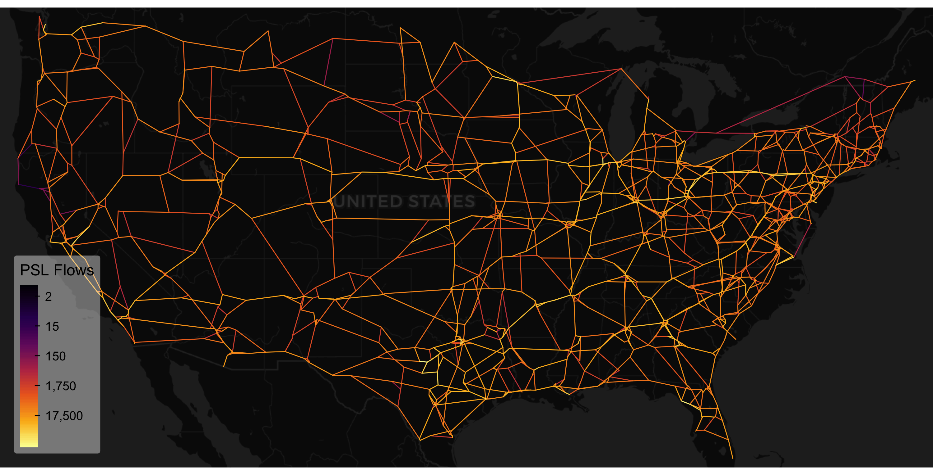
flows_c_sc <- simplify_network(flows_c, zones_agg$NN_undir) |>
  consolidate_graph(keep = zones_agg$NN_undir, w = ~ cost, verbose = FALSE)
## Created graph with 145789 nodes and 229724 edges...
## Retained 32118/229724 edges traversed by shortest paths (14.0%)
nrow(flows_c_sc)
## [1] 3091
And voila, that I would call a radical simplification, first retaining 32,118 edges traversed by shortest paths and then recursively consolidating them down to 3091 edges.
The result is visually sparse, and the simplification discards flows on non-traversed links. Ideally one would re-assign the OD matrix to the simplified network; I leave that as an exercise since the procedure should be clear by now.
A viable alternative retaining far more edges for alternative routing is to base the shortest-path simplification on the full 3796 disaggregated zones rather than only the 132 aggregated zones:
# Need to first match them to the undirected graph
flows_c_nodes <- nodes_from_graph(flows_c, sf = TRUE)
zones$NN_undir <- flows_c_nodes$node[st_nearest_feature(zones, flows_c_nodes)]
# Combining with the aggregate zone nearest nodes
sp_nodes <- unique(c(zones$NN_undir, zones_agg$NN_undir))
length(sp_nodes)
## [1] 3457
# Now simplifying again
flows_c_sc <- simplify_network(flows_c, sp_nodes) |>
   consolidate_graph(keep = zones_agg$NN_undir, w = ~ cost, verbose = FALSE)
## Created graph with 145789 nodes and 229724 edges...
## Retained 107695/229724 edges traversed by shortest paths (46.9%)
nrow(flows_c_sc)
## [1] 48672
The resulting graph is much more detailed. This required computing 3457*(3457-1)/2 = 5,973,696 shortest paths, which took ~3 min—a future update will add multithreading to simplify_network().
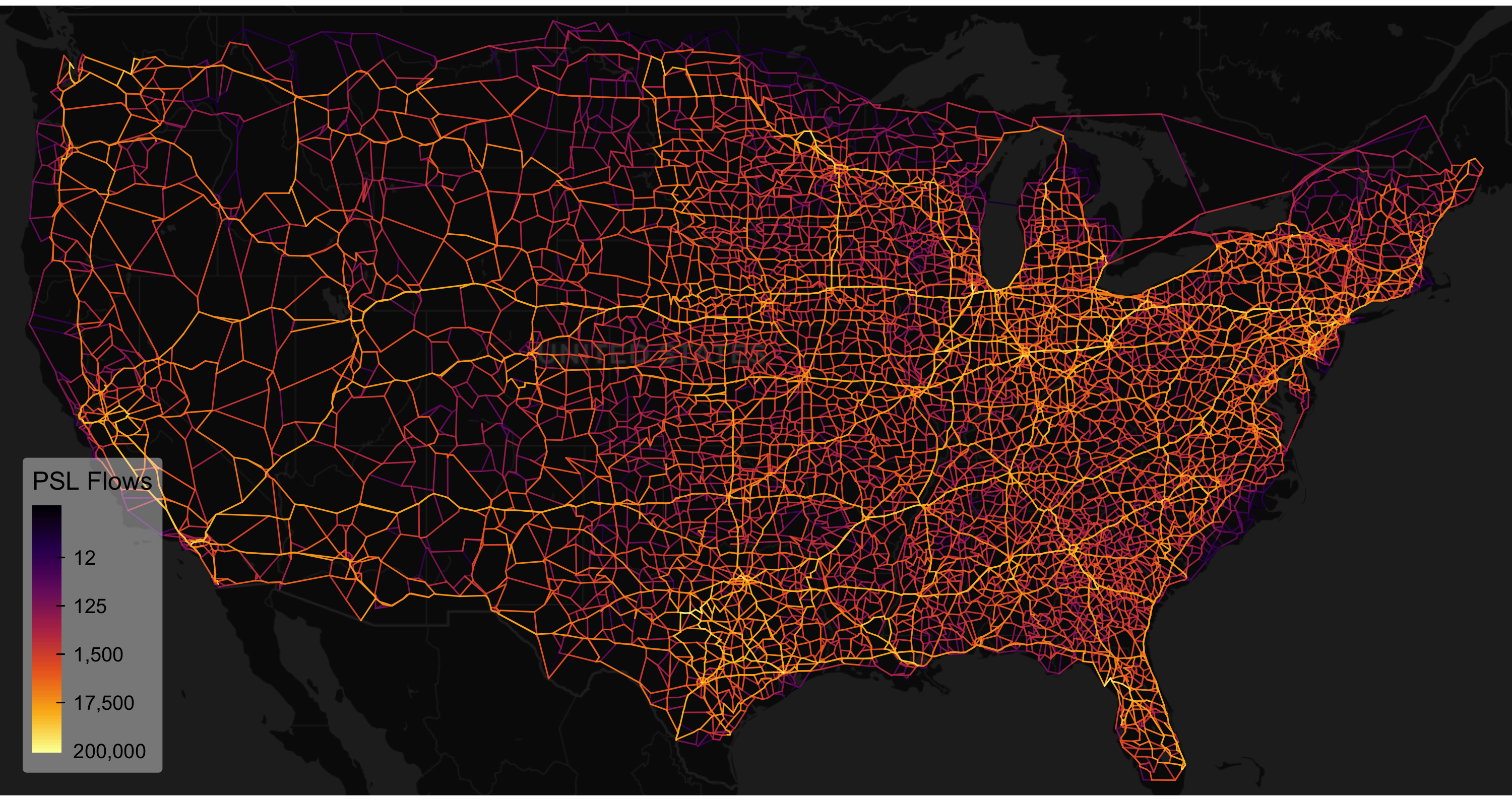
This simplified and consolidated network certainly looks more appealing and provides a reasonable simplification for routing and stochastic traffic assignment using the PSL in this case.
The second method, "cluster", takes a fundamentally different approach: it spatially clusters nearby nodes and contracts the graph accordingly, (1) dropping intra-cluster loop edges and (2) aggregating inter-cluster edges via collap(). Clustering proceeds in two stages: first, optionally, designate key nodes (e.g., zone centroids) as cluster seeds, absorbing all nodes within a specified radius; then, use Hartigan (1975)’s Leader Algorithm—implemented efficiently in C by leaderCluster with geographic coordinate support—to cluster the remaining nodes using a second radius. If no key nodes are provided, all nodes are clustered via the Leader Algorithm.
Below, we use the 132 zone nodes as cluster seeds and a 7km radius for both stages. The larger the radius, the more aggressive the simplification.8
flows_c_cc <- simplify_network(flows_c, zones_agg$NN_undir, method = "cluster",
                      radius_km = list(nodes = 7, cluster = 7), w = ~ flows) |>
   consolidate_graph(keep = zones_agg$NN_undir, w = ~ cost)
## Clustering nodes close to 'keep' nodes using a radius of 7km
## Clustering the remaining nodes with the leaderCluster algorithm using a radius of 7km
## leaderCluster algorithm converged in 13 iterations
## Dropped 183503 self-loop edges (following clustering)
## Oriented 30362 undirected edges
## Contracting 46221 edges down to 26395 edges
## Consolidating undirected graph . with 26395 edges using full recursion
## Initial node degrees:
##    1    2    3    4    5    6    7    8    9   10   11   13
##   55 2349 5358 3197 1709  972  412  163   46   15    3    1
##
## Dropped 54 edges leading to singleton nodes
## Oriented 1129 undirected intermediate edges
## Contracted 2325 intermediate nodes
## Oriented 1 undirected intermediate edges
## Contracted 1 intermediate nodes
## Aggregated 26341 edges down to 23449 edges
## Dropped 2 loop edges
## Oriented 103 undirected intermediate edges
## Contracted 149 intermediate nodes
## Aggregated 23447 edges down to 23293 edges
## Oriented 6 undirected intermediate edges
## Contracted 6 intermediate nodes
## Aggregated 23293 edges down to 23287 edges
## No nodes to contract, returning graph
##
## Consolidated undirected graph . from 26395 edges to 23287 edges (88.2%)
## Final node degrees:
##    1    2    3    4    5    6    7    8    9   10   12
##    1   24 5477 3288 1641  882  330  101   25    9    1
nrow(flows_c_cc)
## [1] 23287
It is notable that clustering leaves less room for follow-up consolidation than shortest-path simplification, which tends to produce long chains of connected edges.
Let’s look at the result:
Also pretty neat—I think—and very similar. Finally, I note that while this network is unimodal, both consolidate_graph() and simplify_network() support multimodal networks—passing mode identifiers to their ‘by’ arguments prevents edges of different modes from being conflated.
Conclusion
flownet is a new R package for transport modeling. It presently provides route enumeration and traffic assignment using the Path-Sized Logit model, powerful tools for network processing, and a parsimonious API. These features make it a compelling choice for transport analytics, particularly in R. The package is built on top of several fastverse libraries and custom C code to ensure high performance.
In this post, I demonstrated the package on African and US road networks, showcasing how to assign trade/traffic flows with the PSL method, and how to investigate/visualize the results. I additionally demonstrated the package’s network simplification tools on the detailed US network.
Future flownet updates may comprise additional traffic assignment methods, more advanced network processing tools, and performance optimizations. But even in its present state, I believe the package is computationally capable of handling most networks we deal with at CPCS and a wide variety of other applications, including modeling on regional or global multimodal transport networks.
References
Ben-Akiva, M., & Bierlaire, M. (1999). Discrete choice methods and their applications to short term travel decisions. In R. W. Hall (Ed.), Handbook of Transportation Science (pp. 5–33). Springer US. https://doi.org/10.1007/978-1-4615-5203-1_2
Cascetta, E. (2001). Transportation systems engineering: Theory and methods. Springer.
Ben-Akiva, M., & Lerman, S. R. (1985). Discrete choice analysis: Theory and application to travel demand. The MIT Press.
Ramming, M. S. (2002). Network knowledge and route choice (Doctoral dissertation). Massachusetts Institute of Technology.
Prato, C. G. (2009). Route choice modeling: Past, present and future research directions. Journal of Choice Modelling, 2(1), 65–100. https://doi.org/10.1016/S1755-5345(13)70005-8
AequilibraE Python Documentation: https://www.aequilibrae.com/develop/python/route_choice/path_size_logit.html
Hartigan, J. A. (1975). Clustering algorithms. John Wiley & Sons, Inc.
Multimodality is principally supported via
byarguments to network processing functions. Passing link-mode identifiers to this argument prevents network simplification/contraction across different modes.↩︎Measured against a straight line from origin to destination node.↩︎
Exempting the shortest path, which is always included and reported first if
return.extra = "paths".↩︎Disaggregating to all 3796 FAF5 zone nodes (e.g., using population weights as in the Africa example) would yield \(3796^2-3796 \approx 14.4\) million OD pairs, requiring roughly \(14.4\text{M}/16.4\text{k} = 876\times\) longer \(\approx\) 6 days on this machine. A 32-core server might bring this down to ~2 days, given that the 4GHz M4 Pro cores used here are state-of-the-art for single-thread performance.↩︎
linestrings_from_graph()is a convenience function to turn theFX,FY,TX, andTYcoordinates into straight linestrings again.↩︎By default, the mean is applied to numeric and the statistical mode to categorical columns. Structural columns (
edge,from,to,FX,FY,TX,TY) are processed separately so that the consolidated graph has a newedgeid and a consistent spatial structure.↩︎The graph has two non-identifier columns:
"cost"and"flows". Passingw = ~ costtocollap()uses costs as weights for a weighted mean of"flows", and by default sums the weights ("cost") themselves. This yields the total cost along contracted edges and the cost-weighted mean of flows.↩︎Note here how I apply the weight trick using
collap()in two different ways: insimplify_network(), I weight by flows, such that, according tocollap()defaults, the flows along edges that we combine are summed and the costs are averaged using the flows as weights. Then, in the following consolidation, I do it the other way around (as before). Think about it and you will hopefully agree with me that that makes sense.↩︎