Efficient estimation of a Dynamic Factor Model via the EM Algorithm - on stationary data with time-invariant system matrices and classical assumptions, while permitting missing data.
Arguments
- X
a
T x nnumeric data matrix or frame of stationary time series. May contain missing values. Note that data is internally standardized (scaled and centered) before estimation.- r
integer. Number of factors.
- p
integer. Number of lags in factor VAR.
- ...
(optional) arguments to
tsnarmimp. The default settings impute internal missing values with a cubic spline and the edges with the median and a 3-period moving average.- idio.ar1
logical. Model observation errors as AR(1) processes: \(e_t = \rho e_{t-1} + v_t\). Note that this substantially increases computation time, and is generally not needed if
nis large (>30). See theoretical vignette for details.- quarterly.vars
character. Names of quarterly variables in
X(if any). Monthly variables should be to the left of the quarterly variables in the data matrix and quarterly observations should be provided every 3rd period.- rQ
character. Restrictions on the state (transition) covariance matrix (Q).
- rR
character. Restrictions on the observation (measurement) covariance matrix (R).
- em.method
character. The implementation of the Expectation Maximization Algorithm used. The options are:
"auto"Automatic selection: "BM"ifanyNA(X), else"DGR"."DGR"The classical EM implementation of Doz, Giannone and Reichlin (2012). This implementation is efficient and quite robust, missing values are removed on a casewise basis in the Kalman Filter and Smoother, but not explicitly accounted for in EM iterations. "BM"The modified EM algorithm of Banbura and Modugno (2014) which also accounts for missing data in the EM iterations. Optimal for datasets with systematically missing data e.g. datasets with ragged edges or series at different frequencies. "none"Performs no EM iterations and just returns the Two-Step estimates from running the data through the Kalman Filter and Smoother once as in Doz, Giannone and Reichlin (2011) (the Kalman Filter is Initialized with system matrices obtained from a regression and VAR on PCA factor estimates). This yields significant performance gains over the iterative methods. Final system matrices are estimated by running a regression and a VAR on the smoothed factors. - min.iter
integer. Minimum number of EM iterations (to ensure a convergence path).
- max.iter
integer. Maximum number of EM iterations.
- tol
numeric. EM convergence tolerance.
- pos.corr
logical. Increase the likelihood that factors correlate positively with the data, by scaling the eigenvectors such that the principal components (used to initialize the Kalman Filter) co-vary positively with the row-means of the standardized data.
- check.increased
logical. Check if likelihood has increased. Passed to
em_converged. IfTRUE, the algorithm only terminates if convergence was reached with decreasing likelihood.
Value
A list-like object of class 'dfm' with the following elements:
X_imp\(T \times n\) matrix with the imputed and standardized (scaled and centered) data—after applying
tsnarmimp. It has attributes attached allowing for reconstruction of the original data:"stats"is a \(n \times 5\) matrix of summary statistics of class "qsu"(seeqsu)."missing"is a \(T \times n\) logical matrix indicating missing or infinite values in the original data (which are imputed in X_imp)."attributes"contains the attributesof the original data input."is.list"is a logical value indicating whether the original data input was a list / data frame. eigeneigen(cov(X_imp)).F_pca\(T \times r\) matrix of principal component factor estimates -
X_imp %*% eigen$vectors.P_0\(r \times r\) initial factor covariance matrix estimate based on PCA results.
F_2s\(T \times r\) matrix two-step factor estimates as in Doz, Giannone and Reichlin (2011) - obtained from running the data through the Kalman Filter and Smoother once, where the Filter is initialized with results from PCA.
P_2s\(r \times r \times T\) covariance matrices of two-step factor estimates.
F_qml\(T \times r\) matrix of quasi-maximum likelihood factor estimates - obtained by iteratively Kalman Filtering and Smoothing the factor estimates until EM convergence.
P_qml\(r \times r \times T\) covariance matrices of QML factor estimates.
A\(r \times rp\) factor transition matrix.
C\(n \times r\) observation matrix.
Q\(r \times r\) state (error) covariance matrix.
R\(n \times n\) observation (error) covariance matrix.
e\(T \times n\) estimates of observation errors \(\textbf{e}_t\). Only available if
idio.ar1 = TRUE.rho\(n \times 1\) estimates of AR(1) coefficients (\(\rho\)) in observation errors: \(e_t = \rho e_{t-1} + v_t\). Only available if
idio.ar1 = TRUE.loglikvector of log-likelihoods - one for each EM iteration. The final value corresponds to the log-likelihood of the reported model.
tolThe numeric convergence tolerance used.
convergedsingle logical valued indicating whether the EM algorithm converged (within
max.iteriterations subject totol).anyNAsingle logical valued indicating whether there were any (internal) missing values in the data (determined after removal of rows with too many missing values). If
FALSE,X_impis simply the original data in matrix form, and does not have the"missing"attribute attached.rm.rowsvector of any cases (rows) that were removed beforehand (subject to
max.missingandna.rm.method). If no cases were removed the slot isNULL.quarterly.varsnames of the quarterly variables (if any).
em.methodThe EM method used.
callcall object obtained from
match.call().
Details
This function efficiently estimates a Dynamic Factor Model with the following classical assumptions:
Linearity
Idiosynchratic measurement (observation) errors (R is diagonal)
No direct relationship between series and lagged factors (ceteris paribus contemporaneous factors)
No relationship between lagged error terms in the either measurement or transition equation (no serial correlation), unless explicitly modeled as AR(1) processes using
idio.ar1 = TRUE.
Factors are allowed to evolve in a \(VAR(p)\) process, and data is internally standardized (scaled and centered) before estimation (removing the need of intercept terms). By assumptions 1-4, this translates into the following dynamic form:
$$\textbf{x}_t = \textbf{C}_0 \textbf{f}_t + \textbf{e}_t \ \sim\ N(\textbf{0}, \textbf{R})$$ $$\textbf{f}_t = \sum_{j=1}^p \textbf{A}_j \textbf{f}_{t-j} + \textbf{u}_t \ \sim\ N(\textbf{0}, \textbf{Q}_0)$$
where the first equation is called the measurement or observation equation and the second equation is called transition, state or process equation, and
| \(n\) | number of series in \(\textbf{x}_t\) (\(r\) and \(p\) as the arguments to DFM). | ||
| \(\textbf{x}_t\) | \(n \times 1\) vector of observed series at time \(t\): \((x_{1t}, \dots, x_{nt})'\). Some observations can be missing. | ||
| \(\textbf{f}_t\) | \(r \times 1\) vector of factors at time \(t\): \((f_{1t}, \dots, f_{rt})'\). | ||
| \(\textbf{C}_0\) | \(n \times r\) measurement (observation) matrix. | ||
| \(\textbf{A}_j\) | \(r \times r\) state transition matrix at lag \(j\). | ||
| \(\textbf{Q}_0\) | \(r \times r\) state covariance matrix. | ||
| \(\textbf{R}\) | \(n \times n\) measurement (observation) covariance matrix. It is diagonal by assumption 2 that \(E[\textbf{x}_{it}|\textbf{x}_{-i,t},\textbf{x}_{i,t-1}, \dots, \textbf{f}_t, \textbf{f}_{t-1}, \dots] = \textbf{Cf}_t \forall i\). |
This model can be estimated using a classical form of the Kalman Filter and the Expectation Maximization (EM) algorithm, after transforming it to State-Space (stacked, VAR(1)) form:
$$\textbf{x}_t = \textbf{C} \textbf{F}_t + \textbf{e}_t \ \sim\ N(\textbf{0}, \textbf{R})$$ $$\textbf{F}_t = \textbf{A F}_{t-1} + \textbf{u}_t \ \sim\ N(\textbf{0}, \textbf{Q})$$
where
| \(n\) | number of series in \(\textbf{x}_t\) (\(r\) and \(p\) as the arguments to DFM). | ||
| \(\textbf{x}_t\) | \(n \times 1\) vector of observed series at time \(t\): \((x_{1t}, \dots, x_{nt})'\). Some observations can be missing. | ||
| \(\textbf{F}_t\) | \(rp \times 1\) vector of stacked factors at time \(t\): \((f_{1t}, \dots, f_{rt}, f_{1,t-1}, \dots, f_{r,t-1}, \dots, f_{1,t-p}, \dots, f_{r,t-p})'\). | ||
| \(\textbf{C}\) | \(n \times rp\) observation matrix. Only the first \(n \times r\) terms are non-zero, by assumption 3 that \(E[\textbf{x}_t|\textbf{F}_t] = E[\textbf{x}_t|\textbf{f}_t]\) (no relationship of observed series with lagged factors given contemporaneous factors). | ||
| \(\textbf{A}\) | stacked \(rp \times rp\) state transition matrix consisting of 3 parts: the top \(r \times rp\) part provides the dynamic relationships captured by \((\textbf{A}_1, \dots, \textbf{A}_p)\) in the dynamic form, the terms A[(r+1):rp, 1:(rp-r)] constitute an \((rp-r) \times (rp-r)\) identity matrix mapping all lagged factors to their known values at times t. The remaining part A[(rp-r+1):rp, (rp-r+1):rp] is an \(r \times r\) matrix of zeros. | ||
| \(\textbf{Q}\) | \(rp \times rp\) state covariance matrix. The top \(r \times r\) part gives the contemporaneous relationships, the rest are zeros by assumption 4. | ||
| \(\textbf{R}\) | \(n \times n\) observation covariance matrix. It is diagonal by assumption 2 and identical to \(\textbf{R}\) as stated in the dynamic form. |
The filter is initialized with PCA estimates on the imputed dataset—see SKFS for a complete code example.
References
Doz, C., Giannone, D., & Reichlin, L. (2011). A two-step estimator for large approximate dynamic factor models based on Kalman filtering. Journal of Econometrics, 164(1), 188-205.
Doz, C., Giannone, D., & Reichlin, L. (2012). A quasi-maximum likelihood approach for large, approximate dynamic factor models. Review of Economics and Statistics, 94(4), 1014-1024.
Banbura, M., & Modugno, M. (2014). Maximum likelihood estimation of factor models on datasets with arbitrary pattern of missing data. Journal of Applied Econometrics, 29(1), 133-160.
Stock, J. H., & Watson, M. W. (2016). Dynamic Factor Models, Factor-Augmented Vector Autoregressions, and Structural Vector Autoregressions in Macroeconomics. Handbook of Macroeconomics, 2, 415–525. https://doi.org/10.1016/bs.hesmac.2016.04.002
Examples
library(magrittr)
library(xts)
library(vars)
#> Loading required package: MASS
#> Loading required package: strucchange
#> Loading required package: sandwich
#> Loading required package: urca
#> Loading required package: lmtest
# BM14 Replication Data. Constructing the database:
BM14 <- merge(BM14_M, BM14_Q)
BM14[, BM14_Models$log_trans] %<>% log()
BM14[, BM14_Models$freq == "M"] %<>% diff()
BM14[, BM14_Models$freq == "Q"] %<>% diff(3)
# \donttest{
### Small Model ---------------------------------------
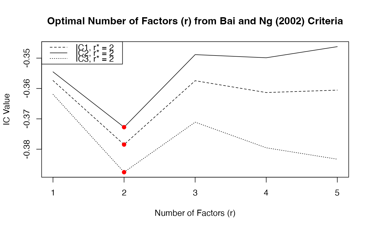
# IC for number of factors
IC_small <- ICr(BM14[, BM14_Models$small], max.r = 5)
#> Missing values detected: imputing data with tsnarmimp() with default settings
plot(IC_small)
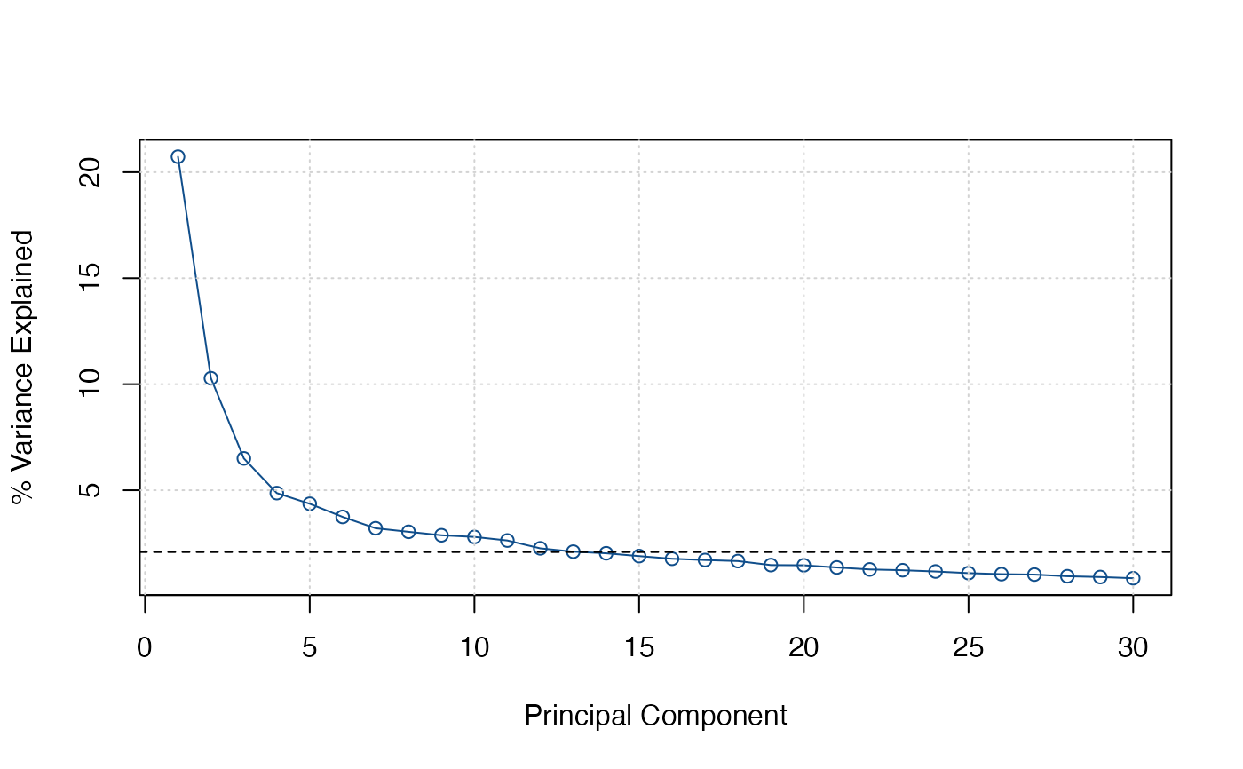
 screeplot(IC_small)
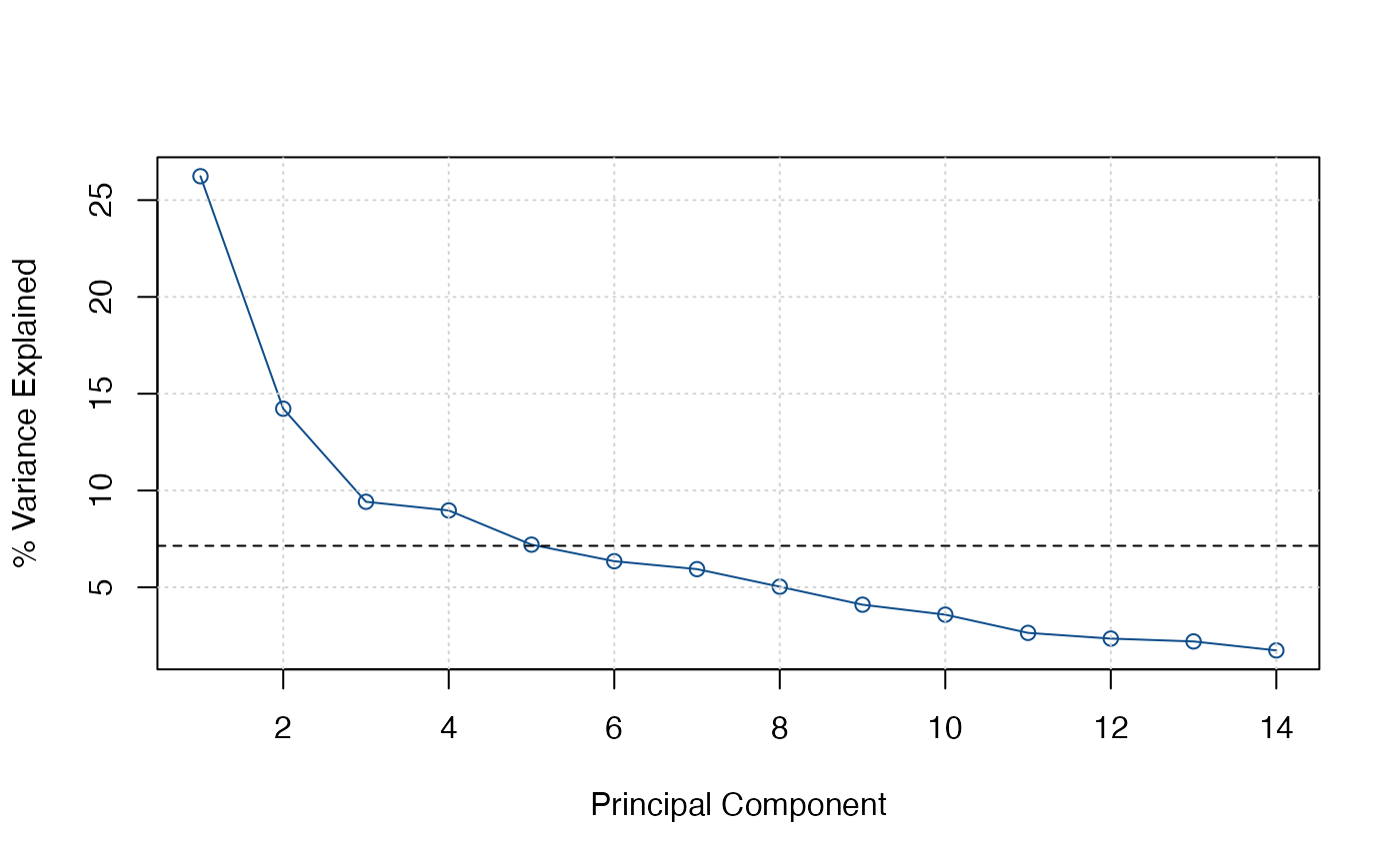 # I take 2 factors. Now number of lags
VARselect(IC_small$F_pca[, 1:2])
#> $selection
#> AIC(n) HQ(n) SC(n) FPE(n)
#> 6 5 2 6
#>
#> $criteria
#> 1 2 3 4 5 6
#> AIC(n) -1.5028163 -1.7020957 -1.701093 -1.7021266 -1.782692 -1.7977899
#> HQ(n) -1.4762557 -1.6578279 -1.639118 -1.6224446 -1.685303 -1.6826936
#> SC(n) -1.4361151 -1.5909270 -1.545457 -1.5020229 -1.538121 -1.5087511
#> FPE(n) 0.2225028 0.1823018 0.182486 0.1822997 0.168192 0.1656763
#> 7 8 9 10
#> AIC(n) -1.7892503 -1.7887748 -1.7793434 -1.7708400
#> HQ(n) -1.6564469 -1.6382643 -1.6111258 -1.5849153
#> SC(n) -1.4557440 -1.4108011 -1.3569022 -1.3039313
#> FPE(n) 0.1671036 0.1671913 0.1687862 0.1702408
#>
# Estimating the model with 2 factors and 3 lags
dfm_small <- DFM(BM14[, BM14_Models$small], r = 2, p = 3,
quarterly.vars = BM14_Models %$% series[freq == "Q" & small])
#> Converged after 26 iterations.
# Inspecting the model
summary(dfm_small)
#> Mixed Frequency Dynamic Factor Model
#> n = 14, nm = 10, nq = 4, T = 356, r = 2, p = 3
#> %NA = 38.3628, %NAm = 26.3202
#>
#> Call: DFM(X = BM14[, BM14_Models$small], r = 2, p = 3, quarterly.vars = BM14_Models %$% series[freq == "Q" & small])
#>
#> Summary Statistics of Factors [F]
#> N Mean Median SD Min Max
#> f1 356 -0.1605 0.1274 2.0755 -9.4638 3.1838
#> f2 356 0.1049 0.0463 1.3905 -4.2535 5.3709
#>
#> Factor Transition Matrix [A]
#> L1.f1 L1.f2 L2.f1 L2.f2 L3.f1 L3.f2
#> f1 1.2824 -0.1946 -0.2100 0.2179 -0.1402 -0.05373
#> f2 0.1709 0.5829 0.2514 -0.2866 -0.6082 0.41312
#>
#> Factor Covariance Matrix [cov(F)]
#> f1 f2
#> f1 4.3077 -0.5272*
#> f2 -0.5272* 1.9334
#>
#> Factor Transition Error Covariance Matrix [Q]
#> u1 u2
#> u1 0.3026 0.2191
#> u2 0.2191 0.4764
#>
#> Observation Matrix [C]
#> f1 f2
#> ip_tot_cstr 0.2516 0.1905
#> new_cars 0.0265 0.0290
#> orders 0.1725 0.1659
#> ret_turnover_defl 0.0533 0.0067
#> ecs_ec_sent_ind 0.2650 0.4645
#> pms_pmi 0.1296 0.4786
#> urx -0.3799 0.1838
#> extra_ea_trade_exp_val 0.0601 0.0865
#> euro325 0.1307 0.2383
#> raw_mat 0.0958 0.1625
#> gdp 0.0434 0.0217
#> empl 0.0437 -0.0249
#> capacity 0.0392 0.0116
#> gdp_us 0.0268 0.0437
#>
#> Observation Error Covariance Matrix [diag(R) - Restricted]
#> ip_tot_cstr new_cars orders
#> 0.6269 0.9909 0.7924
#> ret_turnover_defl ecs_ec_sent_ind pms_pmi
#> 0.9845 0.3332 0.3706
#> urx extra_ea_trade_exp_val euro325
#> 0.1681 0.9688 0.8183
#> raw_mat gdp empl
#> 0.9096 0.3599 0.1326
#> capacity gdp_us
#> 0.4659 0.6048
#>
#> Observation Residual Covariance Matrix [cov(resid(DFM))]
#> ip_tot_cstr new_cars orders ret_turnover_defl
#> ip_tot_cstr 0.6016 -0.0155 0.1950* -0.0191
#> new_cars -0.0155 0.9946 -0.0080 0.1262
#> orders 0.1950* -0.0080 0.7821 0.0324
#> ret_turnover_defl -0.0191 0.1262 0.0324 0.9864
#> ecs_ec_sent_ind -0.0209 -0.0282 -0.0861* -0.0101
#> pms_pmi -0.0687 -0.0472 -0.0187 0.0022
#> urx 0.0113 -0.0158 0.0547* -0.0098
#> extra_ea_trade_exp_val 0.0697 0.0963 0.0742 -0.0190
#> euro325 -0.0373 0.0556 -0.0904 0.0107
#> raw_mat 0.0921 0.1067 0.0067 0.0323
#> gdp 0.0720 -0.0844 0.0107 -0.0055
#> empl -0.0031 -0.1102 -0.0405 -0.0695
#> capacity -0.0066 -0.0474 -0.0520 -0.1209
#> gdp_us -0.0740 -0.0115 0.0609 -0.1050
#> ecs_ec_sent_ind pms_pmi urx
#> ip_tot_cstr -0.0209 -0.0687 0.0113
#> new_cars -0.0282 -0.0472 -0.0158
#> orders -0.0861* -0.0187 0.0547*
#> ret_turnover_defl -0.0101 0.0022 -0.0098
#> ecs_ec_sent_ind 0.2434 -0.0836* -0.0114
#> pms_pmi -0.0836* 0.2982 0.0106
#> urx -0.0114 0.0106 0.1409
#> extra_ea_trade_exp_val -0.0697* -0.0419 0.0077
#> euro325 -0.0358 -0.0396 -0.0014
#> raw_mat -0.0433 0.0339 0.0248
#> gdp -0.0258 0.0604 0.0200
#> empl 0.0444 0.1233 0.0351
#> capacity -0.0473 0.0574 0.0304
#> gdp_us -0.0519 0.0210 0.0555
#> extra_ea_trade_exp_val euro325 raw_mat gdp
#> ip_tot_cstr 0.0697 -0.0373 0.0921 0.0720
#> new_cars 0.0963 0.0556 0.1067 -0.0844
#> orders 0.0742 -0.0904 0.0067 0.0107
#> ret_turnover_defl -0.0190 0.0107 0.0323 -0.0055
#> ecs_ec_sent_ind -0.0697* -0.0358 -0.0433 -0.0258
#> pms_pmi -0.0419 -0.0396 0.0339 0.0604
#> urx 0.0077 -0.0014 0.0248 0.0200
#> extra_ea_trade_exp_val 0.9673 0.0112 -0.0329 0.0482
#> euro325 0.0112 0.7982 0.0097 0.0341
#> raw_mat -0.0329 0.0097 0.8984 0.0022
#> gdp 0.0482 0.0341 0.0022 0.8794
#> empl -0.0869 0.0905 0.0372 0.4779*
#> capacity -0.0428 0.0477 -0.1930* 0.5392*
#> gdp_us -0.0780 0.1076 0.0037 0.3432*
#> empl capacity gdp_us
#> ip_tot_cstr -0.0031 -0.0066 -0.0740
#> new_cars -0.1102 -0.0474 -0.0115
#> orders -0.0405 -0.0520 0.0609
#> ret_turnover_defl -0.0695 -0.1209 -0.1050
#> ecs_ec_sent_ind 0.0444 -0.0473 -0.0519
#> pms_pmi 0.1233 0.0574 0.0210
#> urx 0.0351 0.0304 0.0555
#> extra_ea_trade_exp_val -0.0869 -0.0428 -0.0780
#> euro325 0.0905 0.0477 0.1076
#> raw_mat 0.0372 -0.1930* 0.0037
#> gdp 0.4779* 0.5392* 0.3432*
#> empl 0.8218 0.4565* 0.1683*
#> capacity 0.4565* 0.9166 0.2969*
#> gdp_us 0.1683* 0.2969* 0.9371
#>
#> Residual AR(1) Serial Correlation
#> ip_tot_cstr new_cars orders
#> -0.38749 -0.40829 -0.41500
#> ret_turnover_defl ecs_ec_sent_ind pms_pmi
#> -0.49326 -0.09350 0.08832
#> urx extra_ea_trade_exp_val euro325
#> -0.09171 -0.52651 0.24433
#> raw_mat gdp empl
#> 0.27610 NA NA
#> capacity gdp_us
#> NA NA
#>
#> Summary of Residual AR(1) Serial Correlations
#> N Mean Median SD Min Max
#> 10 -0.1807 -0.2405 0.3062 -0.5265 0.2761
#>
#> Goodness of Fit: R-Squared
#> ip_tot_cstr new_cars orders
#> 0.3984 0.0054 0.2179
#> ret_turnover_defl ecs_ec_sent_ind pms_pmi
#> 0.0136 0.7566 0.7018
#> urx extra_ea_trade_exp_val euro325
#> 0.8591 0.0327 0.2018
#> raw_mat gdp empl
#> 0.1016 0.1206 0.1782
#> capacity gdp_us
#> 0.0834 0.0629
#>
#> Summary of Individual R-Squared's
#> N Mean Median SD Min Max
#> 14 0.2667 0.1494 0.2939 0.0054 0.8591
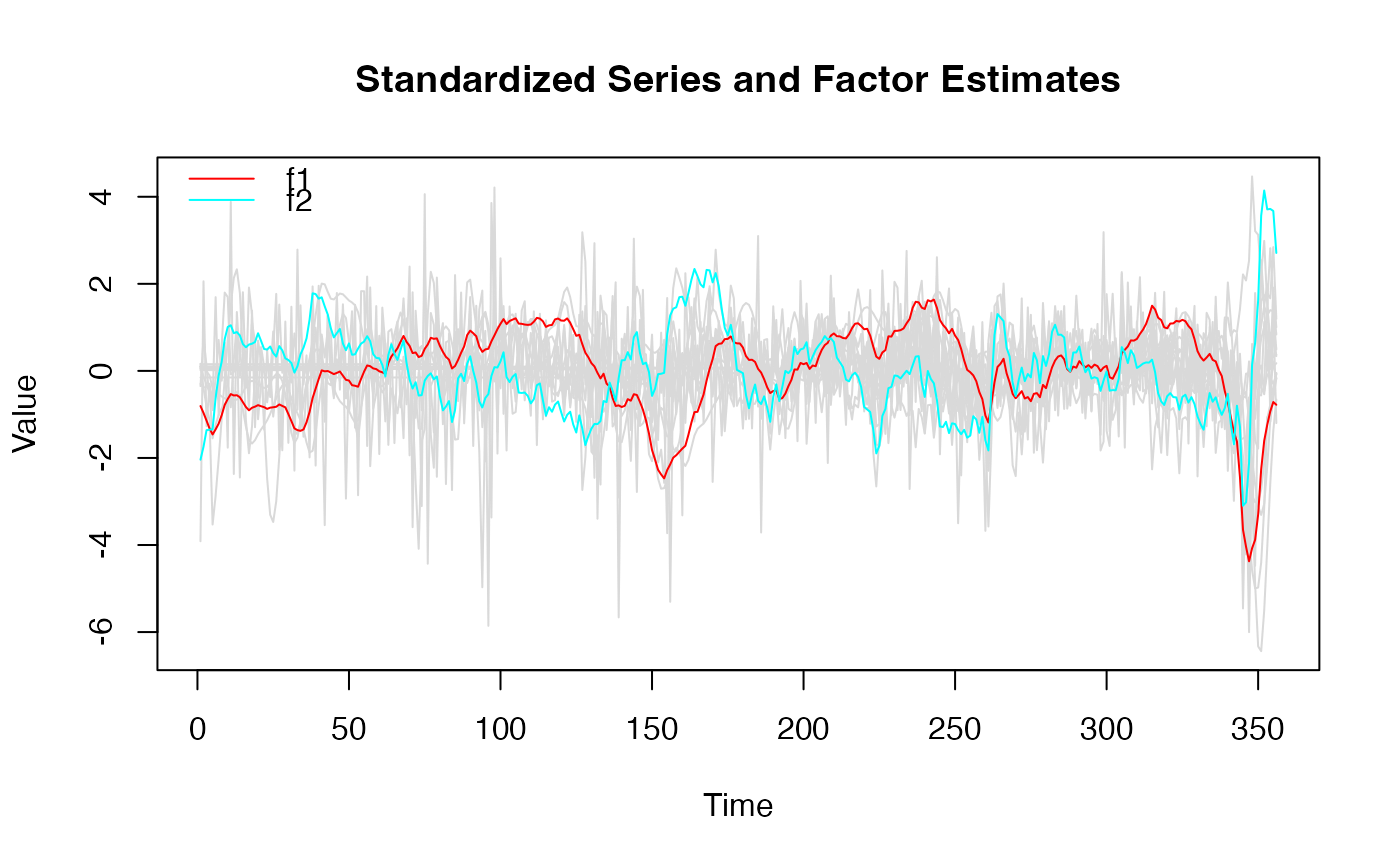
plot(dfm_small) # Factors and data
# I take 2 factors. Now number of lags
VARselect(IC_small$F_pca[, 1:2])
#> $selection
#> AIC(n) HQ(n) SC(n) FPE(n)
#> 6 5 2 6
#>
#> $criteria
#> 1 2 3 4 5 6
#> AIC(n) -1.5028163 -1.7020957 -1.701093 -1.7021266 -1.782692 -1.7977899
#> HQ(n) -1.4762557 -1.6578279 -1.639118 -1.6224446 -1.685303 -1.6826936
#> SC(n) -1.4361151 -1.5909270 -1.545457 -1.5020229 -1.538121 -1.5087511
#> FPE(n) 0.2225028 0.1823018 0.182486 0.1822997 0.168192 0.1656763
#> 7 8 9 10
#> AIC(n) -1.7892503 -1.7887748 -1.7793434 -1.7708400
#> HQ(n) -1.6564469 -1.6382643 -1.6111258 -1.5849153
#> SC(n) -1.4557440 -1.4108011 -1.3569022 -1.3039313
#> FPE(n) 0.1671036 0.1671913 0.1687862 0.1702408
#>
# Estimating the model with 2 factors and 3 lags
dfm_small <- DFM(BM14[, BM14_Models$small], r = 2, p = 3,
quarterly.vars = BM14_Models %$% series[freq == "Q" & small])
#> Converged after 26 iterations.
# Inspecting the model
summary(dfm_small)
#> Mixed Frequency Dynamic Factor Model
#> n = 14, nm = 10, nq = 4, T = 356, r = 2, p = 3
#> %NA = 38.3628, %NAm = 26.3202
#>
#> Call: DFM(X = BM14[, BM14_Models$small], r = 2, p = 3, quarterly.vars = BM14_Models %$% series[freq == "Q" & small])
#>
#> Summary Statistics of Factors [F]
#> N Mean Median SD Min Max
#> f1 356 -0.1605 0.1274 2.0755 -9.4638 3.1838
#> f2 356 0.1049 0.0463 1.3905 -4.2535 5.3709
#>
#> Factor Transition Matrix [A]
#> L1.f1 L1.f2 L2.f1 L2.f2 L3.f1 L3.f2
#> f1 1.2824 -0.1946 -0.2100 0.2179 -0.1402 -0.05373
#> f2 0.1709 0.5829 0.2514 -0.2866 -0.6082 0.41312
#>
#> Factor Covariance Matrix [cov(F)]
#> f1 f2
#> f1 4.3077 -0.5272*
#> f2 -0.5272* 1.9334
#>
#> Factor Transition Error Covariance Matrix [Q]
#> u1 u2
#> u1 0.3026 0.2191
#> u2 0.2191 0.4764
#>
#> Observation Matrix [C]
#> f1 f2
#> ip_tot_cstr 0.2516 0.1905
#> new_cars 0.0265 0.0290
#> orders 0.1725 0.1659
#> ret_turnover_defl 0.0533 0.0067
#> ecs_ec_sent_ind 0.2650 0.4645
#> pms_pmi 0.1296 0.4786
#> urx -0.3799 0.1838
#> extra_ea_trade_exp_val 0.0601 0.0865
#> euro325 0.1307 0.2383
#> raw_mat 0.0958 0.1625
#> gdp 0.0434 0.0217
#> empl 0.0437 -0.0249
#> capacity 0.0392 0.0116
#> gdp_us 0.0268 0.0437
#>
#> Observation Error Covariance Matrix [diag(R) - Restricted]
#> ip_tot_cstr new_cars orders
#> 0.6269 0.9909 0.7924
#> ret_turnover_defl ecs_ec_sent_ind pms_pmi
#> 0.9845 0.3332 0.3706
#> urx extra_ea_trade_exp_val euro325
#> 0.1681 0.9688 0.8183
#> raw_mat gdp empl
#> 0.9096 0.3599 0.1326
#> capacity gdp_us
#> 0.4659 0.6048
#>
#> Observation Residual Covariance Matrix [cov(resid(DFM))]
#> ip_tot_cstr new_cars orders ret_turnover_defl
#> ip_tot_cstr 0.6016 -0.0155 0.1950* -0.0191
#> new_cars -0.0155 0.9946 -0.0080 0.1262
#> orders 0.1950* -0.0080 0.7821 0.0324
#> ret_turnover_defl -0.0191 0.1262 0.0324 0.9864
#> ecs_ec_sent_ind -0.0209 -0.0282 -0.0861* -0.0101
#> pms_pmi -0.0687 -0.0472 -0.0187 0.0022
#> urx 0.0113 -0.0158 0.0547* -0.0098
#> extra_ea_trade_exp_val 0.0697 0.0963 0.0742 -0.0190
#> euro325 -0.0373 0.0556 -0.0904 0.0107
#> raw_mat 0.0921 0.1067 0.0067 0.0323
#> gdp 0.0720 -0.0844 0.0107 -0.0055
#> empl -0.0031 -0.1102 -0.0405 -0.0695
#> capacity -0.0066 -0.0474 -0.0520 -0.1209
#> gdp_us -0.0740 -0.0115 0.0609 -0.1050
#> ecs_ec_sent_ind pms_pmi urx
#> ip_tot_cstr -0.0209 -0.0687 0.0113
#> new_cars -0.0282 -0.0472 -0.0158
#> orders -0.0861* -0.0187 0.0547*
#> ret_turnover_defl -0.0101 0.0022 -0.0098
#> ecs_ec_sent_ind 0.2434 -0.0836* -0.0114
#> pms_pmi -0.0836* 0.2982 0.0106
#> urx -0.0114 0.0106 0.1409
#> extra_ea_trade_exp_val -0.0697* -0.0419 0.0077
#> euro325 -0.0358 -0.0396 -0.0014
#> raw_mat -0.0433 0.0339 0.0248
#> gdp -0.0258 0.0604 0.0200
#> empl 0.0444 0.1233 0.0351
#> capacity -0.0473 0.0574 0.0304
#> gdp_us -0.0519 0.0210 0.0555
#> extra_ea_trade_exp_val euro325 raw_mat gdp
#> ip_tot_cstr 0.0697 -0.0373 0.0921 0.0720
#> new_cars 0.0963 0.0556 0.1067 -0.0844
#> orders 0.0742 -0.0904 0.0067 0.0107
#> ret_turnover_defl -0.0190 0.0107 0.0323 -0.0055
#> ecs_ec_sent_ind -0.0697* -0.0358 -0.0433 -0.0258
#> pms_pmi -0.0419 -0.0396 0.0339 0.0604
#> urx 0.0077 -0.0014 0.0248 0.0200
#> extra_ea_trade_exp_val 0.9673 0.0112 -0.0329 0.0482
#> euro325 0.0112 0.7982 0.0097 0.0341
#> raw_mat -0.0329 0.0097 0.8984 0.0022
#> gdp 0.0482 0.0341 0.0022 0.8794
#> empl -0.0869 0.0905 0.0372 0.4779*
#> capacity -0.0428 0.0477 -0.1930* 0.5392*
#> gdp_us -0.0780 0.1076 0.0037 0.3432*
#> empl capacity gdp_us
#> ip_tot_cstr -0.0031 -0.0066 -0.0740
#> new_cars -0.1102 -0.0474 -0.0115
#> orders -0.0405 -0.0520 0.0609
#> ret_turnover_defl -0.0695 -0.1209 -0.1050
#> ecs_ec_sent_ind 0.0444 -0.0473 -0.0519
#> pms_pmi 0.1233 0.0574 0.0210
#> urx 0.0351 0.0304 0.0555
#> extra_ea_trade_exp_val -0.0869 -0.0428 -0.0780
#> euro325 0.0905 0.0477 0.1076
#> raw_mat 0.0372 -0.1930* 0.0037
#> gdp 0.4779* 0.5392* 0.3432*
#> empl 0.8218 0.4565* 0.1683*
#> capacity 0.4565* 0.9166 0.2969*
#> gdp_us 0.1683* 0.2969* 0.9371
#>
#> Residual AR(1) Serial Correlation
#> ip_tot_cstr new_cars orders
#> -0.38749 -0.40829 -0.41500
#> ret_turnover_defl ecs_ec_sent_ind pms_pmi
#> -0.49326 -0.09350 0.08832
#> urx extra_ea_trade_exp_val euro325
#> -0.09171 -0.52651 0.24433
#> raw_mat gdp empl
#> 0.27610 NA NA
#> capacity gdp_us
#> NA NA
#>
#> Summary of Residual AR(1) Serial Correlations
#> N Mean Median SD Min Max
#> 10 -0.1807 -0.2405 0.3062 -0.5265 0.2761
#>
#> Goodness of Fit: R-Squared
#> ip_tot_cstr new_cars orders
#> 0.3984 0.0054 0.2179
#> ret_turnover_defl ecs_ec_sent_ind pms_pmi
#> 0.0136 0.7566 0.7018
#> urx extra_ea_trade_exp_val euro325
#> 0.8591 0.0327 0.2018
#> raw_mat gdp empl
#> 0.1016 0.1206 0.1782
#> capacity gdp_us
#> 0.0834 0.0629
#>
#> Summary of Individual R-Squared's
#> N Mean Median SD Min Max
#> 14 0.2667 0.1494 0.2939 0.0054 0.8591
plot(dfm_small) # Factors and data
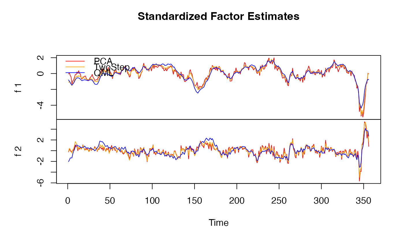
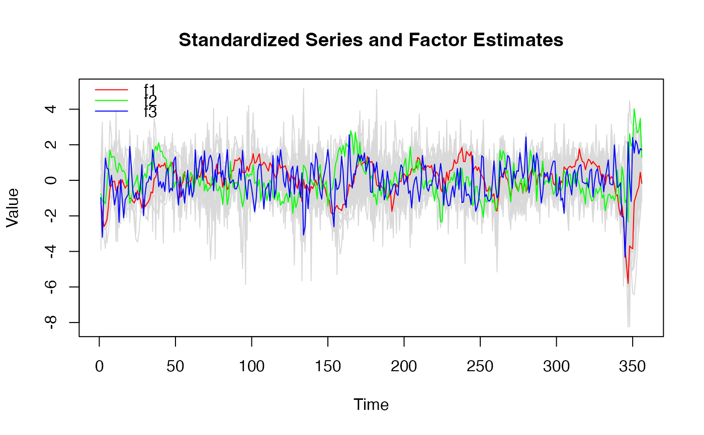
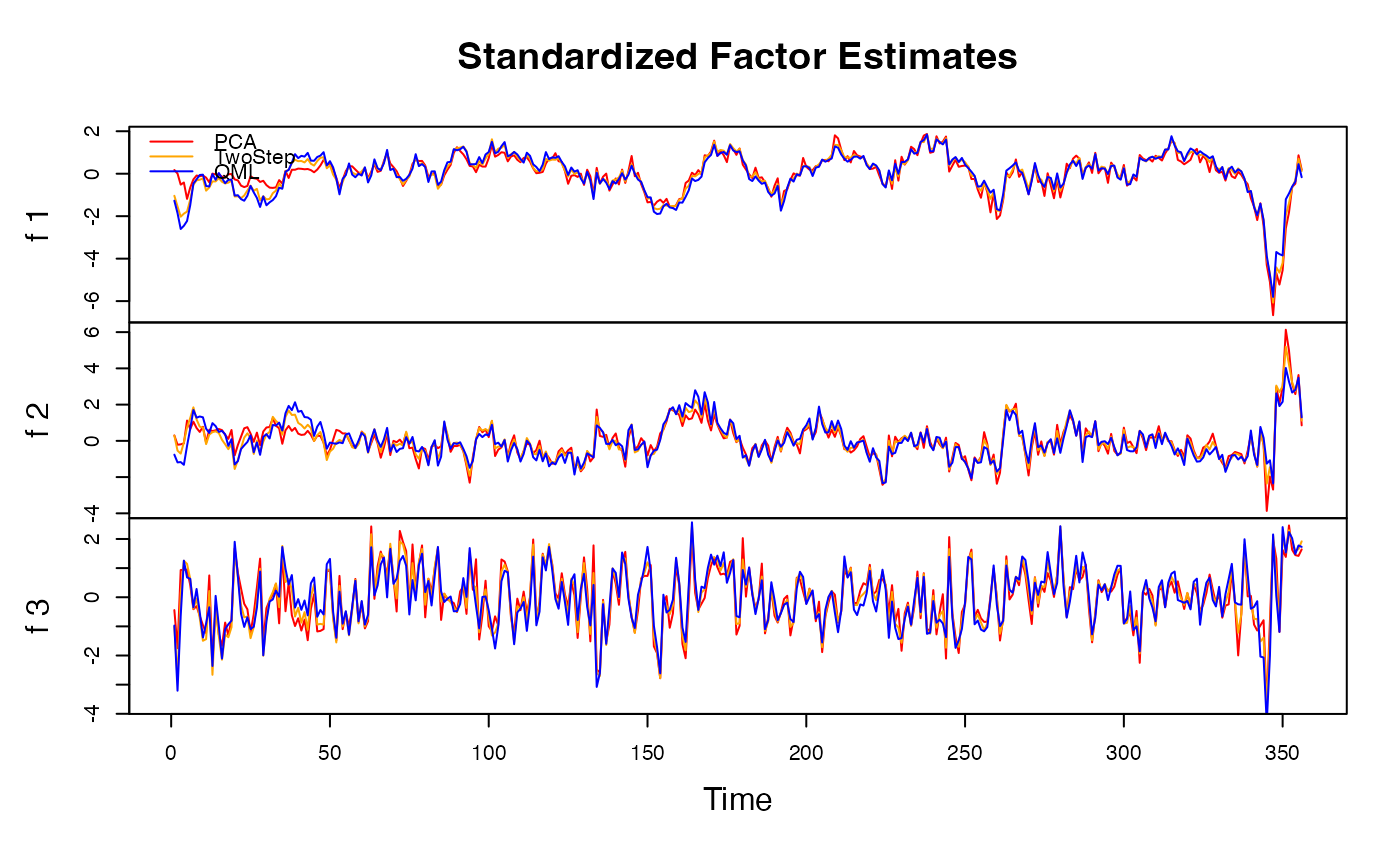
 plot(dfm_small, method = "all", type = "individual") # Factor estimates
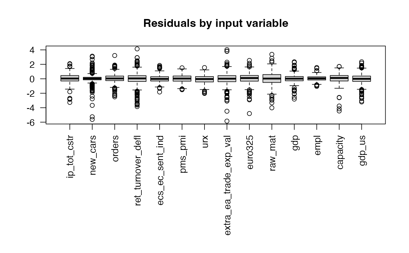
 plot(dfm_small, type = "residual") # Residuals from factor predictions
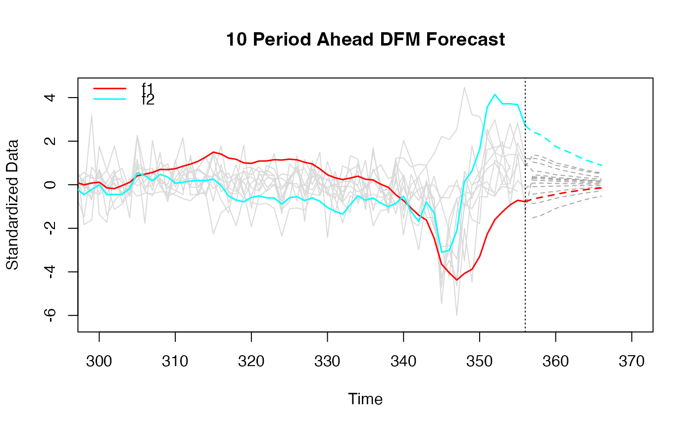
 # 10 periods ahead forecast
plot(predict(dfm_small), xlim = c(300, 370))
# 10 periods ahead forecast
plot(predict(dfm_small), xlim = c(300, 370))
 ### Medium-Sized Model ---------------------------------
# IC for number of factors
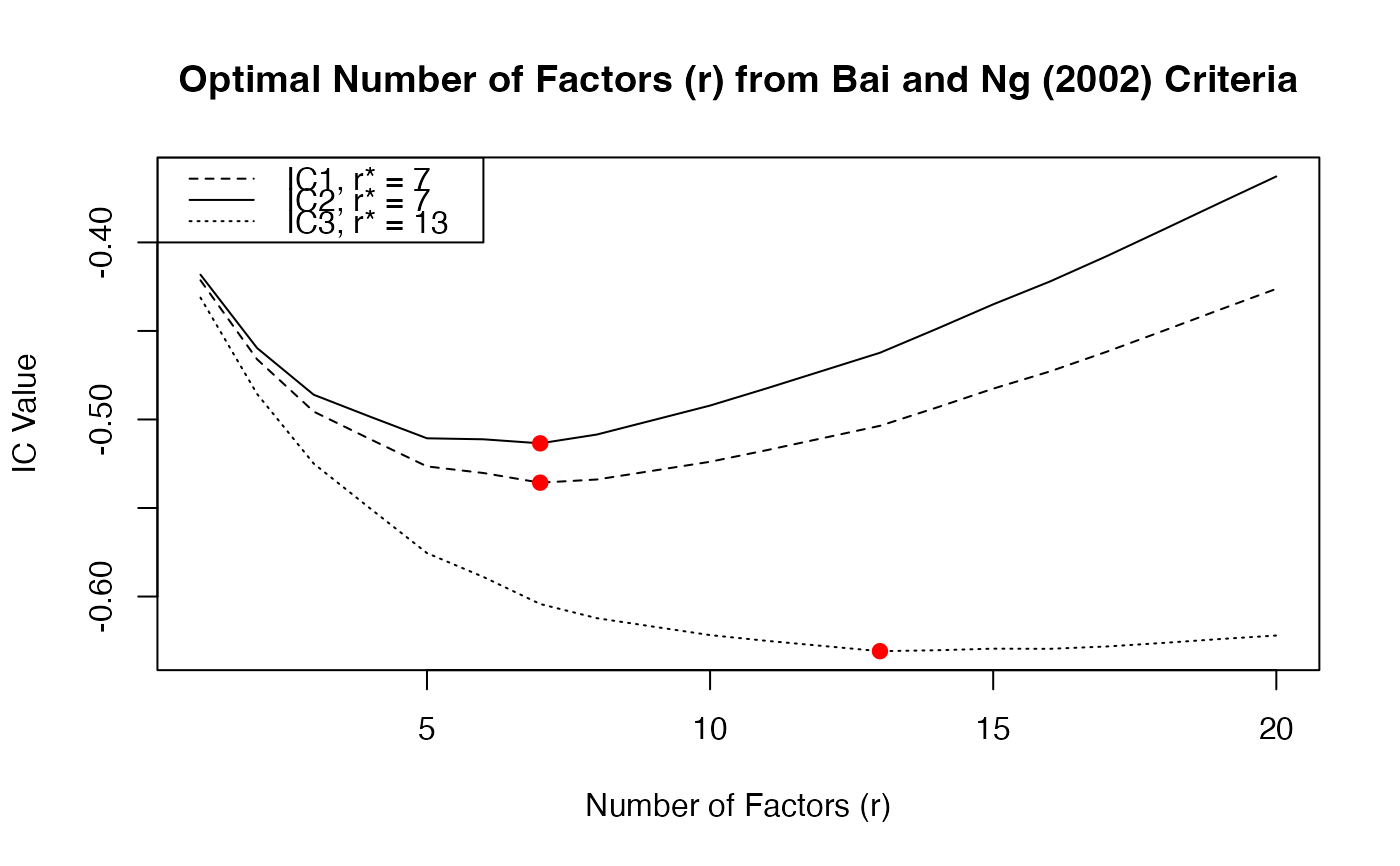
IC_medium <- ICr(BM14[, BM14_Models$medium])
#> Missing values detected: imputing data with tsnarmimp() with default settings
plot(IC_medium)
### Medium-Sized Model ---------------------------------
# IC for number of factors
IC_medium <- ICr(BM14[, BM14_Models$medium])
#> Missing values detected: imputing data with tsnarmimp() with default settings
plot(IC_medium)
 screeplot(IC_medium)
 # I take 3 factors. Now number of lags
VARselect(IC_medium$F_pca[, 1:3])
#> $selection
#> AIC(n) HQ(n) SC(n) FPE(n)
#> 7 2 1 7
#>
#> $criteria
#> 1 2 3 4 5 6 7 8
#> AIC(n) 1.539267 1.492781 1.498671 1.509014 1.486111 1.479450 1.468524 1.490378
#> HQ(n) 1.592388 1.585744 1.631474 1.681659 1.698597 1.731776 1.760691 1.822386
#> SC(n) 1.672669 1.726236 1.832177 1.942573 2.019721 2.113112 2.202238 2.324143
#> FPE(n) 4.661186 4.449528 4.475952 4.522752 4.420750 4.391987 4.345059 4.442132
#> 9 10
#> AIC(n) 1.500199 1.534401
#> HQ(n) 1.872048 1.946092
#> SC(n) 2.434016 2.568271
#> FPE(n) 4.487352 4.645257
#>
# Estimating the model with 3 factors and 3 lags
dfm_medium <- DFM(BM14[, BM14_Models$medium], r = 3, p = 3,
quarterly.vars = BM14_Models %$% series[freq == "Q" & medium])
#> Converged after 26 iterations.
# Inspecting the model
summary(dfm_medium)
#> Mixed Frequency Dynamic Factor Model
#> n = 48, nm = 39, nq = 9, T = 356, r = 3, p = 3
#> %NA = 32.6135, %NAm = 24.0781
#>
#> Call: DFM(X = BM14[, BM14_Models$medium], r = 3, p = 3, quarterly.vars = BM14_Models %$% series[freq == "Q" & medium])
#>
#> Summary Statistics of Factors [F]
#> N Mean Median SD Min Max
#> f1 356 -0.0985 0.4918 3.1283 -19.3582 5.3549
#> f2 356 0.0341 -0.224 2.2831 -6.462 8.3411
#> f3 356 -0.0172 -0.1399 1.5726 -6.7371 4.3577
#>
#> Factor Transition Matrix [A]
#> L1.f1 L1.f2 L1.f3 L2.f1 L2.f2 L2.f3 L3.f1 L3.f2 L3.f3
#> f1 0.93895 -0.19728 0.1715 0.05318 0.06486 0.01496 -0.1298 0.0859 -0.02337
#> f2 -0.30923 0.75786 0.1641 0.38513 -0.38768 -0.02307 -0.2750 0.4086 0.02054
#> f3 0.06881 0.03244 0.4077 0.36873 -0.32608 -0.17889 -0.4565 0.3461 0.11805
#>
#> Factor Covariance Matrix [cov(F)]
#> f1 f2 f3
#> f1 9.7864 -0.6567 0.3212
#> f2 -0.6567 5.2124 0.0848
#> f3 0.3212 0.0848 2.4729
#>
#> Factor Transition Error Covariance Matrix [Q]
#> u1 u2 u3
#> u1 1.8586 1.3143 -0.3865
#> u2 1.3143 1.8104 -0.5786
#> u3 -0.3865 -0.5786 1.8320
#>
#> Summary of Residual AR(1) Serial Correlations
#> N Mean Median SD Min Max
#> 39 -0.0901 -0.0699 0.2595 -0.5508 0.3205
#>
#> Summary of Individual R-Squared's
#> N Mean Median SD Min Max
#> 48 0.2894 0.155 0.2852 0.0086 0.9362
plot(dfm_medium) # Factors and data
# I take 3 factors. Now number of lags
VARselect(IC_medium$F_pca[, 1:3])
#> $selection
#> AIC(n) HQ(n) SC(n) FPE(n)
#> 7 2 1 7
#>
#> $criteria
#> 1 2 3 4 5 6 7 8
#> AIC(n) 1.539267 1.492781 1.498671 1.509014 1.486111 1.479450 1.468524 1.490378
#> HQ(n) 1.592388 1.585744 1.631474 1.681659 1.698597 1.731776 1.760691 1.822386
#> SC(n) 1.672669 1.726236 1.832177 1.942573 2.019721 2.113112 2.202238 2.324143
#> FPE(n) 4.661186 4.449528 4.475952 4.522752 4.420750 4.391987 4.345059 4.442132
#> 9 10
#> AIC(n) 1.500199 1.534401
#> HQ(n) 1.872048 1.946092
#> SC(n) 2.434016 2.568271
#> FPE(n) 4.487352 4.645257
#>
# Estimating the model with 3 factors and 3 lags
dfm_medium <- DFM(BM14[, BM14_Models$medium], r = 3, p = 3,
quarterly.vars = BM14_Models %$% series[freq == "Q" & medium])
#> Converged after 26 iterations.
# Inspecting the model
summary(dfm_medium)
#> Mixed Frequency Dynamic Factor Model
#> n = 48, nm = 39, nq = 9, T = 356, r = 3, p = 3
#> %NA = 32.6135, %NAm = 24.0781
#>
#> Call: DFM(X = BM14[, BM14_Models$medium], r = 3, p = 3, quarterly.vars = BM14_Models %$% series[freq == "Q" & medium])
#>
#> Summary Statistics of Factors [F]
#> N Mean Median SD Min Max
#> f1 356 -0.0985 0.4918 3.1283 -19.3582 5.3549
#> f2 356 0.0341 -0.224 2.2831 -6.462 8.3411
#> f3 356 -0.0172 -0.1399 1.5726 -6.7371 4.3577
#>
#> Factor Transition Matrix [A]
#> L1.f1 L1.f2 L1.f3 L2.f1 L2.f2 L2.f3 L3.f1 L3.f2 L3.f3
#> f1 0.93895 -0.19728 0.1715 0.05318 0.06486 0.01496 -0.1298 0.0859 -0.02337
#> f2 -0.30923 0.75786 0.1641 0.38513 -0.38768 -0.02307 -0.2750 0.4086 0.02054
#> f3 0.06881 0.03244 0.4077 0.36873 -0.32608 -0.17889 -0.4565 0.3461 0.11805
#>
#> Factor Covariance Matrix [cov(F)]
#> f1 f2 f3
#> f1 9.7864 -0.6567 0.3212
#> f2 -0.6567 5.2124 0.0848
#> f3 0.3212 0.0848 2.4729
#>
#> Factor Transition Error Covariance Matrix [Q]
#> u1 u2 u3
#> u1 1.8586 1.3143 -0.3865
#> u2 1.3143 1.8104 -0.5786
#> u3 -0.3865 -0.5786 1.8320
#>
#> Summary of Residual AR(1) Serial Correlations
#> N Mean Median SD Min Max
#> 39 -0.0901 -0.0699 0.2595 -0.5508 0.3205
#>
#> Summary of Individual R-Squared's
#> N Mean Median SD Min Max
#> 48 0.2894 0.155 0.2852 0.0086 0.9362
plot(dfm_medium) # Factors and data
 plot(dfm_medium, method = "all", type = "individual") # Factor estimates
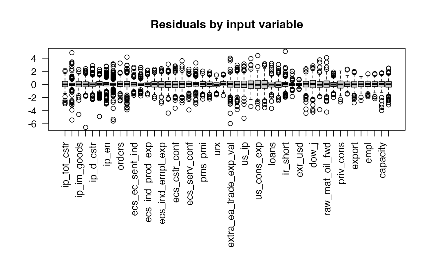
 plot(dfm_medium, type = "residual") # Residuals from factor predictions
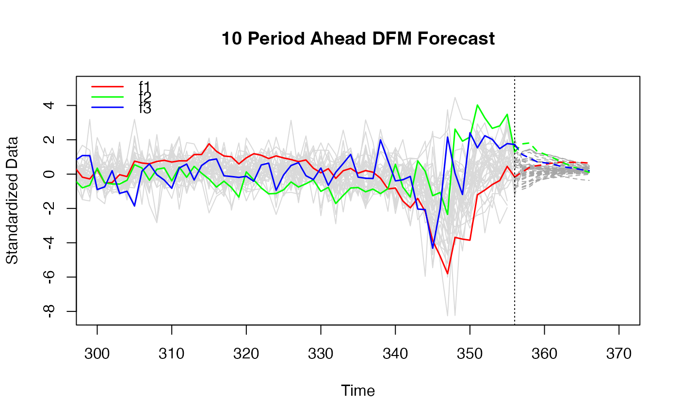
 # 10 periods ahead forecast
plot(predict(dfm_medium), xlim = c(300, 370))
# 10 periods ahead forecast
plot(predict(dfm_medium), xlim = c(300, 370))
 ### Large Model ---------------------------------
# IC for number of factors
IC_large <- ICr(BM14)
#> Missing values detected: imputing data with tsnarmimp() with default settings
plot(IC_large)
### Large Model ---------------------------------
# IC for number of factors
IC_large <- ICr(BM14)
#> Missing values detected: imputing data with tsnarmimp() with default settings
plot(IC_large)
 screeplot(IC_large)
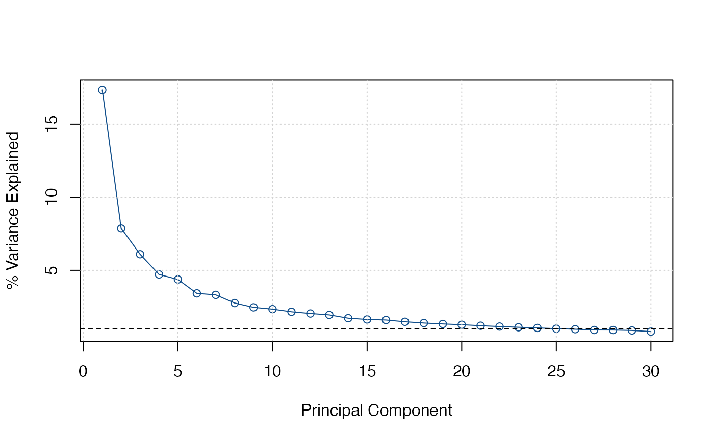 # I take 6 factors. Now number of lags
VARselect(IC_large$F_pca[, 1:6])
#> $selection
#> AIC(n) HQ(n) SC(n) FPE(n)
#> 6 1 1 6
#>
#> $criteria
#> 1 2 3 4 5 6
#> AIC(n) 6.020768 5.926947 5.883307 5.889824 5.897327 5.845883
#> HQ(n) 6.206692 6.272235 6.387960 6.553841 6.720708 6.828628
#> SC(n) 6.487677 6.794063 7.150631 7.557355 7.965066 8.313830
#> FPE(n) 411.908362 375.087393 359.232802 361.888929 365.116976 347.515300
#> 7 8 9 10
#> AIC(n) 5.908082 5.963699 5.982969 6.111831
#> HQ(n) 7.050191 7.265172 7.443806 7.732032
#> SC(n) 8.776235 9.232061 9.651538 10.180607
#> FPE(n) 370.862536 393.546431 403.139879 461.355079
#>
# Estimating the model with 6 factors and 3 lags
dfm_large <- DFM(BM14, r = 6, p = 3,
quarterly.vars = BM14_Models %$% series[freq == "Q"])
#> Converged after 39 iterations.
# Inspecting the model
summary(dfm_large)
#> Mixed Frequency Dynamic Factor Model
#> n = 101, nm = 92, nq = 9, T = 356, r = 6, p = 3
#> %NA = 29.7363, %NAm = 25.8366
#>
#> Call: DFM(X = BM14, r = 6, p = 3, quarterly.vars = BM14_Models %$% series[freq == "Q"])
#>
#> Summary Statistics of Factors [F]
#> N Mean Median SD Min Max
#> f1 356 -0.107 0.6573 4.8387 -23.1251 14.7986
#> f2 356 -0.2216 0.1847 3.4756 -13.9892 17.5939
#> f3 356 -0.0085 0.038 2.538 -9.952 7.023
#> f4 356 0.1225 0.2815 3.1901 -17.2132 11.1281
#> f5 356 -0.0816 -0.0857 2.6977 -11.8225 11.6105
#> f6 356 -0.0021 -0.0044 2.2638 -8.0332 14.3884
#>
#> Factor Transition Matrix [A]
#> L1.f1 L1.f2 L1.f3 L1.f4 L1.f5 L1.f6 L2.f1 L2.f2
#> f1 0.4146 -0.31547 0.535594 -0.409677 0.24935 -0.042001 -0.0013023 0.10535
#> f2 -0.1181 0.42170 -0.132113 -0.044417 0.11608 0.126305 0.0865712 -0.02060
#> f3 0.2563 0.07508 0.387405 0.069762 -0.13764 -0.102988 -0.1223568 0.01331
#> f4 -0.2962 -0.12730 0.098611 -0.104417 0.48309 -0.037316 0.0466138 -0.10279
#> f5 0.3225 0.08940 -0.008011 0.344206 0.09136 0.009044 -0.0134199 0.07329
#> f6 -0.1849 0.10457 -0.088462 -0.009701 -0.07510 0.362577 0.0007091 -0.06256
#> L2.f3 L2.f4 L2.f5 L2.f6 L3.f1 L3.f2 L3.f3 L3.f4
#> f1 -0.18944 -0.17725 -0.036033 0.48920 0.32166 -0.06934 0.06825 0.05621
#> f2 0.04108 -0.06438 0.172166 -0.08944 0.15363 0.22166 0.11864 -0.13273
#> f3 -0.27139 0.19914 -0.010737 0.02744 -0.04957 -0.08776 0.10569 0.12061
#> f4 0.04184 -0.17465 -0.003223 0.16731 0.07214 -0.11843 -0.03447 0.12219
#> f5 -0.08275 -0.01601 -0.107952 -0.10232 -0.17649 0.02642 -0.00477 0.01682
#> f6 0.03254 -0.04805 0.086758 -0.10416 0.09119 0.06214 0.13715 -0.12928
#> L3.f5 L3.f6
#> f1 0.15754 0.05201
#> f2 0.01799 0.09386
#> f3 -0.11424 0.01713
#> f4 -0.06460 0.07272
#> f5 0.03395 -0.14320
#> f6 0.05089 0.02547
#>
#> Factor Covariance Matrix [cov(F)]
#> f1 f2 f3 f4 f5 f6
#> f1 23.4128 0.7031 -0.2198 3.7881* -2.5178* -1.9928*
#> f2 0.7031 12.0798 -1.6485* -0.4811 -0.6676 2.4008*
#> f3 -0.2198 -1.6485* 6.4415 -1.4691* 1.4553* -0.9491*
#> f4 3.7881* -0.4811 -1.4691* 10.1768 -4.6435* -0.4141
#> f5 -2.5178* -0.6676 1.4553* -4.6435* 7.2774 -0.4585
#> f6 -1.9928* 2.4008* -0.9491* -0.4141 -0.4585 5.1250
#>
#> Factor Transition Error Covariance Matrix [Q]
#> u1 u2 u3 u4 u5 u6
#> u1 10.2115 0.2060 -1.4420 2.4061 -2.2408 0.2968
#> u2 0.2060 5.8639 -0.0814 0.8044 -0.6562 0.1438
#> u3 -1.4420 -0.0814 4.3219 -0.5280 0.4627 0.1162
#> u4 2.4061 0.8044 -0.5280 4.9253 -1.6502 0.0570
#> u5 -2.2408 -0.6562 0.4627 -1.6502 4.4696 -0.0469
#> u6 0.2968 0.1438 0.1162 0.0570 -0.0469 3.1868
#>
#> Summary of Residual AR(1) Serial Correlations
#> N Mean Median SD Min Max
#> 92 -0.0673 -0.0953 0.2657 -0.4957 0.6614
#>
#> Summary of Individual R-Squared's
#> N Mean Median SD Min Max
#> 101 0.4297 0.3892 0.3071 0.0121 0.9987
plot(dfm_large) # Factors and data
# I take 6 factors. Now number of lags
VARselect(IC_large$F_pca[, 1:6])
#> $selection
#> AIC(n) HQ(n) SC(n) FPE(n)
#> 6 1 1 6
#>
#> $criteria
#> 1 2 3 4 5 6
#> AIC(n) 6.020768 5.926947 5.883307 5.889824 5.897327 5.845883
#> HQ(n) 6.206692 6.272235 6.387960 6.553841 6.720708 6.828628
#> SC(n) 6.487677 6.794063 7.150631 7.557355 7.965066 8.313830
#> FPE(n) 411.908362 375.087393 359.232802 361.888929 365.116976 347.515300
#> 7 8 9 10
#> AIC(n) 5.908082 5.963699 5.982969 6.111831
#> HQ(n) 7.050191 7.265172 7.443806 7.732032
#> SC(n) 8.776235 9.232061 9.651538 10.180607
#> FPE(n) 370.862536 393.546431 403.139879 461.355079
#>
# Estimating the model with 6 factors and 3 lags
dfm_large <- DFM(BM14, r = 6, p = 3,
quarterly.vars = BM14_Models %$% series[freq == "Q"])
#> Converged after 39 iterations.
# Inspecting the model
summary(dfm_large)
#> Mixed Frequency Dynamic Factor Model
#> n = 101, nm = 92, nq = 9, T = 356, r = 6, p = 3
#> %NA = 29.7363, %NAm = 25.8366
#>
#> Call: DFM(X = BM14, r = 6, p = 3, quarterly.vars = BM14_Models %$% series[freq == "Q"])
#>
#> Summary Statistics of Factors [F]
#> N Mean Median SD Min Max
#> f1 356 -0.107 0.6573 4.8387 -23.1251 14.7986
#> f2 356 -0.2216 0.1847 3.4756 -13.9892 17.5939
#> f3 356 -0.0085 0.038 2.538 -9.952 7.023
#> f4 356 0.1225 0.2815 3.1901 -17.2132 11.1281
#> f5 356 -0.0816 -0.0857 2.6977 -11.8225 11.6105
#> f6 356 -0.0021 -0.0044 2.2638 -8.0332 14.3884
#>
#> Factor Transition Matrix [A]
#> L1.f1 L1.f2 L1.f3 L1.f4 L1.f5 L1.f6 L2.f1 L2.f2
#> f1 0.4146 -0.31547 0.535594 -0.409677 0.24935 -0.042001 -0.0013023 0.10535
#> f2 -0.1181 0.42170 -0.132113 -0.044417 0.11608 0.126305 0.0865712 -0.02060
#> f3 0.2563 0.07508 0.387405 0.069762 -0.13764 -0.102988 -0.1223568 0.01331
#> f4 -0.2962 -0.12730 0.098611 -0.104417 0.48309 -0.037316 0.0466138 -0.10279
#> f5 0.3225 0.08940 -0.008011 0.344206 0.09136 0.009044 -0.0134199 0.07329
#> f6 -0.1849 0.10457 -0.088462 -0.009701 -0.07510 0.362577 0.0007091 -0.06256
#> L2.f3 L2.f4 L2.f5 L2.f6 L3.f1 L3.f2 L3.f3 L3.f4
#> f1 -0.18944 -0.17725 -0.036033 0.48920 0.32166 -0.06934 0.06825 0.05621
#> f2 0.04108 -0.06438 0.172166 -0.08944 0.15363 0.22166 0.11864 -0.13273
#> f3 -0.27139 0.19914 -0.010737 0.02744 -0.04957 -0.08776 0.10569 0.12061
#> f4 0.04184 -0.17465 -0.003223 0.16731 0.07214 -0.11843 -0.03447 0.12219
#> f5 -0.08275 -0.01601 -0.107952 -0.10232 -0.17649 0.02642 -0.00477 0.01682
#> f6 0.03254 -0.04805 0.086758 -0.10416 0.09119 0.06214 0.13715 -0.12928
#> L3.f5 L3.f6
#> f1 0.15754 0.05201
#> f2 0.01799 0.09386
#> f3 -0.11424 0.01713
#> f4 -0.06460 0.07272
#> f5 0.03395 -0.14320
#> f6 0.05089 0.02547
#>
#> Factor Covariance Matrix [cov(F)]
#> f1 f2 f3 f4 f5 f6
#> f1 23.4128 0.7031 -0.2198 3.7881* -2.5178* -1.9928*
#> f2 0.7031 12.0798 -1.6485* -0.4811 -0.6676 2.4008*
#> f3 -0.2198 -1.6485* 6.4415 -1.4691* 1.4553* -0.9491*
#> f4 3.7881* -0.4811 -1.4691* 10.1768 -4.6435* -0.4141
#> f5 -2.5178* -0.6676 1.4553* -4.6435* 7.2774 -0.4585
#> f6 -1.9928* 2.4008* -0.9491* -0.4141 -0.4585 5.1250
#>
#> Factor Transition Error Covariance Matrix [Q]
#> u1 u2 u3 u4 u5 u6
#> u1 10.2115 0.2060 -1.4420 2.4061 -2.2408 0.2968
#> u2 0.2060 5.8639 -0.0814 0.8044 -0.6562 0.1438
#> u3 -1.4420 -0.0814 4.3219 -0.5280 0.4627 0.1162
#> u4 2.4061 0.8044 -0.5280 4.9253 -1.6502 0.0570
#> u5 -2.2408 -0.6562 0.4627 -1.6502 4.4696 -0.0469
#> u6 0.2968 0.1438 0.1162 0.0570 -0.0469 3.1868
#>
#> Summary of Residual AR(1) Serial Correlations
#> N Mean Median SD Min Max
#> 92 -0.0673 -0.0953 0.2657 -0.4957 0.6614
#>
#> Summary of Individual R-Squared's
#> N Mean Median SD Min Max
#> 101 0.4297 0.3892 0.3071 0.0121 0.9987
plot(dfm_large) # Factors and data
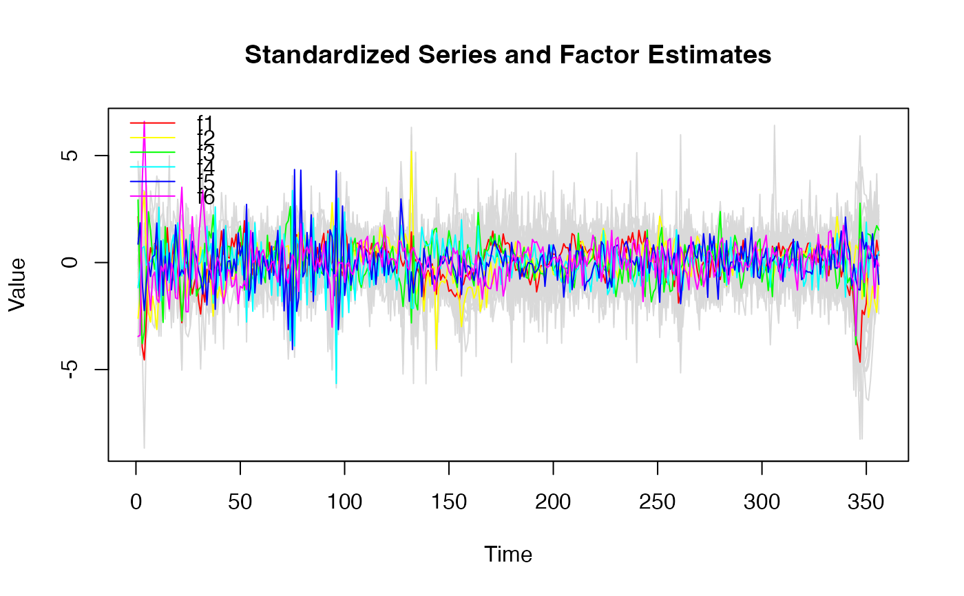 # plot(dfm_large, method = "all", type = "individual") # Factor estimates
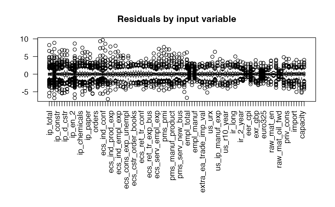
plot(dfm_large, type = "residual") # Residuals from factor predictions
# plot(dfm_large, method = "all", type = "individual") # Factor estimates
plot(dfm_large, type = "residual") # Residuals from factor predictions
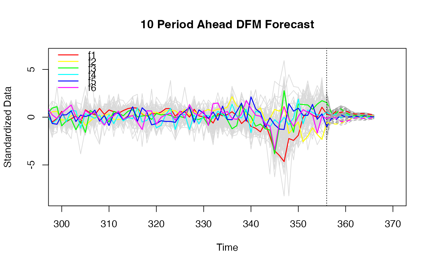
 # 10 periods ahead forecast
plot(predict(dfm_large), xlim = c(300, 370))
# 10 periods ahead forecast
plot(predict(dfm_large), xlim = c(300, 370))
 # }
# }