The Past

collapse started in 2019 as a small package with only two functions: collap() - intended to facilitate the aggregation of mixed-type data in R, and qsu() - intended to facilitate summarizing panel data in R. Both were inspired by STATA’s collapse and (xt)summarize commands, and implemented with data.table as a backend. The package - called collapse alluding to the STATA command - would probably have stayed this way, had not unforeseen events affected my career plans.

Having completed a master’s in international economics in summer 2019, I was preparing for a two-year posting as an ODI Fellow in the Central Bank of Papua New Guinea in fall. However, things did not work out, I had difficulties getting a working visa and there were coordination issues with the Bank, so ODI decided to offer me a posting in the Ugandan Ministry of Finance, starting in January 2020. This gave me 4 months, September-December 2019, during which I ended up writing a new backend for collapse - in C++.

While collapse with data.table backed was never particularly slow, some of the underlying metaprogramming seemed arcane, especially because I wanted to utilize data.table’s GeForce optimizations which require the aggregation function to be recognizable in the call for data.table to internally replace it with an optimized version. But there were also statistical limitations. As an economist, I often employed sampling or trade weights in statistics, and in this respect, R was quite limited. There was also no straightforward way to aggregate categorical data, using, as I would have it, a (weighted) statistical mode function. I also felt R was lacking basic things in the time series domain - evidenced by the lengths I went to handle (irregular) trade panels. Finally, I felt limited by the division of software development around different classes in R. I found data.table useful for analytics, but the class too complex to behave in predictable ways. Thus I often ended up converting back to ‘data.frame’ or ‘tibble’ to use functions from a different package. Sometimes it would also have been practical to simply keep data as a vector or matrix - in linear-algebra-heavy programs - but I needed data.table to do something ‘by groups’. So in short, my workflow in R employed frequent object conversions, faced statistical limitations, and, in the case of early collapse’s data.table backend, also involved tedious metaprogramming.

The will for change pushed me to practically rethink the way statistics could be done in R. It required a framework that encompassed increased statistical complexity, including advanced statistical algorithms like (weighted) medians, quantiles, modes, support for (irregular) time series and panels etc., and enabling these operations to be vectored efficiently across many groups and columns without a limiting syntax that would again encourage metaprogramming. The framework would also need to be class-agnostic/support multiple R objects and classes, to easily integrate with different frameworks and reduce the need for object conversions. These considerations led to the creation of a comprehensive set of S3 generic grouped and weighted Fast Statistical Functions for vectors matrices and data.frame-like objects, initially programmed fully in C++. The functions natively supported R factors for grouping. To facilitate programming further, I created multivariate grouping (‘GRP’) objects that could be used to perform multiple statistical operations across the same groups without grouping overhead. With this backend and hand, it was easy to reimplement collap()¹, and also provide a whole array of other useful functions, including dplyr-like functions like fgroup_by(), and time series functions that could be used ad-hoc but also supported plm’s indexed ‘pseries’ and ‘pdata.frame’ classes. collapse 1.0.0, released to CRAN on 19th March 2020 (me sitting in the Ugandan finance ministry) was already a substantial piece of statistical software offering cutting-edge performance (see the benchmarks in the introductory blog post).

To then cut a long story short, in the coming 3 years collapse became better, broader, and faster in multiple iterations. Additional speed came especially from rewriting central parts of the package in C - reimplementing some core algorithms in C rather than relying on the C++ standard library or Rcpp sugar - as well as introducing data transformation by reference and OpenMP multithreading. For example, fmode(), rewritten from C++ to C for v1.8.0 (May 2022), became about 3x faster in serial mode (grouped execution), with additional gains through multithreading across groups. Other noteworthy functionality was a modern reimplementation of ‘pseries’ and ‘pdata.frame’, through ‘indexed_frame’ and ‘indexed_series’ classes, fully fledged fsummarise(), fmutate() and across() functions enabling tidyverse-like programming with vectorization for Fast Statistical Functions in the backend, a set of functions facilitating memory efficient R programming and low-cost data object conversions, functions to effectively deal with (nested) lists of data objects - such as unlisting to data frame with unlist2d(), and additional descriptive statistical tools like qtab() and descr(). Particularly 2022 has seen two major updates: v1.7 and v1.8, and the bulk of development for 1.9 - released in January 2023. In improving collapse, I always took inspiration from other packages, most notably data.table, kit, dplyr, fixest, and R itself, to which I am highly indebted. The presentation of collapse at UseR 2022 in June 2022 marks another milestone of its establishment in the R community.

While using R and improving collapse, I became increasingly aware that I was not alone in the pursuit of making R faster and statistically more powerful. Apart from well-established packages like data.table, matrixStats, and fst, I noticed and started using many smaller packages like kit, roll, stringfish, qs, Rfast, coop, fastmap, fasttime, rrapply etc. aimed at improving particular aspects of R in a statistical or computational sense, often offering clean C or C++ implementations with few R-level dependencies. I saw a pattern of common traits and development efforts that were largely complimentary and needed encouragement. My impression at the time - largely unaltered today - was that such efforts were ignored by large parts of the R user community. One reason is of course the lack of visibility and coordination, compared to institutional stakeholders like Rstudio and H2O backing the tidyverse and data.table. Another consideration, it seemed to me, was that the tidyverse is particularly popular simply because there exists an R package and website called tidyverse which loads a set of packages that work well together, and thus alleviates users of the burden of searching CRAN and choosing their own collection of data manipulation packages.

Thus I decided in early 2021 to also create a meta package and GitHub repo called fastverse and use it to promote high-performance R packages with few dependencies. The first version 0.1.6 made it to CRAN in August 2021, attaching 6 core packages (data.table, collapse, matrixStats, kit, fst and magrittr), and allowing easy extension with additional packages using the fastverse_extend() function. With 7 total dependencies instead of 80, it was a considerably more lightweight and computationally powerful alternative to the tidyverse. The README of the GitHub repository has grown largely due to suggestions from the community and now lists many of the highest performing and (mostly) lightweight R packages. Over time I also introduced more useful functionality into the fastverse package, such as the ability to configure the environment and set of packages included using a .fastverse file, an option to install missing packages on the fly, and the fastverse_child() function to create wholly separate package verses. Observing my own frequent usage of data.table, collapse, kit, and magrittr in combination, I did a poll on Twitter in Fall 2022 suggesting the removal of matrixStats and fst from the core set of packages - which as accepted and implemented from v0.3.0 (November 2022). The fastverse package has thus become an extremely lightweight, customizable, and fast tidyverse alternative.

The Present

Today, both collapse and fastverse are well established in a part of the R community closer to econometrics and high-performance statistics. A growing number of econometric packages benefit from collapse as a computational backend, most notably the well-known plm package - which experienced order-of-magnitude performance gains. I am also developing dfms (first CRAN release October 2022), demonstrating that very efficient estimation of Dynamic Factor Models is possible in R combining collapse and RcppArmadillo. collapse is also powering various shiny apps across the web. I ended up creating a collapse-powered public macroeconomic data portal for Uganda, and later, at the Kiel Institute for the World Economy, for Africa at large.

So collapse has made it into production in my own work and the work of others. Core benefits in my experience are that it is lightweight to install on a server, has very low baseline function execution speeds (of a few microseconds instead of milliseconds with most other frameworks) making for speedy reaction times, scales very well to large data, and supports multiple R objects and modes of programming - reducing the need for metaprogramming. Since my own work and the work of others depends on it, API stability has always been important. collapse has not seen any major API changes in updates v1.7-v1.9, and currently no further API changes are planned. This lightweight and robust nature - characteristic of all core fastverse packages esp. data.table - stands in contrast to dplyr, who’s core API involving summarise(), mutate() and across() keeps changing to an extent that at some point in 2022 I removed unit tests of fsummarise() and fmutate() against the dplyr versions from CRAN.

Apart from development, it has also been very fun using the fastverse in the wild for some research projects. Lately, I’ve been working a lot with geospatial data, where the fastverse has enabled numerous interesting applications.

For example, I was interested in how the area of OSM buildings needs to be scaled using a power weight to correlate optimally with nightlights luminosity within a million cells of populated places in Sub-Saharan Africa. Having extracted around 12 million buildings from OSM, I programmed the following objective function and optimized it for power weights between 0.0001 and 5.

library(fastverse)       
library(microbenchmark)

a <- abs(rnorm(12e6, 100, 100))            # Think of this as building areas in m^2
g <- GRP(sample.int(1e6, 12e6, TRUE))      # Think of this as grid cells
y <- fsum(a^1.5, g, use.g.names = FALSE) + # Think of this as nightlights 
     rnorm(g$N.groups, sd = 10000)  
length(y)
## [1] 999989

# Objective function
cor_ay <- function(w, a, y) {
  aw_agg = fsum(a^w, g, use.g.names = FALSE, na.rm = FALSE)
  cor(aw_agg, y) 
}

# Checking the speed of the objective
microbenchmark(cor_ay(2, a, y))
## Unit: milliseconds
##             expr      min      lq     mean   median       uq      max neval
##  cor_ay(2, a, y) 30.42331 32.1136 35.02078 34.43118 36.75326 55.36505   100

# Now the optimization
system.time(res <- optimise(cor_ay, c(0.0001, 5), a, y, maximum = TRUE))
##    user  system elapsed 
##   1.375   0.051   1.427
res
## $maximum
## [1] 1.501067
## 
## $objective
## [1] 0.5792703

The speed of the objective due to GRP() and fsum()² allowed further subdivision of buildings into different classes, and experimentation with finer spatial resolutions.

Another recent application involved finding the 100 nearest neighbors for each of around 100,000 cells (rows) in a rich geospatial dataset with about 50 variables (columns), and estimating a simple proximity-weighted linear regression of an outcome of interest y on a variable of interest z. Since computing a distance matrix on 100,000 rows up-front is infeasible memory-wise, I needed to go row-by-row. Here functions dapply(), fdist() and flm() from collapse, and topn() from kit became very handy.

# Generating the data
X <- rnorm(5e6)       # 100,000 x 50 matrix of characteristics
dim(X) <- c(1e5, 50)
z <- rnorm(1e5)       # Characteristic of interest
y <- z + rnorm(1e5)   # Outcome of interest
Xm <- t(forwardsolve(t(chol(cov(X))), t(X)))    # Transform X to compute Mahalanobis distance (takes account of correlations)

# Coefficients for a single row
coef_i <- function(row_i) {
    mdist = fdist(Xm, row_i, nthreads = 2L)                           # Mahalanobis distance
    best_idx = topn(mdist, 101L, hasna = FALSE, decreasing = FALSE)   # 100 closest points
    best_idx = best_idx[mdist[best_idx] > 0]                          # Removing the point itself (mdist = 0)
    weights = 1 / mdist[best_idx]                                     # Distance weights
    flm(y[best_idx], z[best_idx], weights, add.icpt = TRUE)           # Weighted lm coefficients
}

# Benchmarking a single execution
microbenchmark(coef_i(Xm[1L, ]))
## Unit: microseconds
##              expr     min      lq     mean  median       uq      max neval
##  coef_i(Xm[1L, ]) 927.051 965.591 1149.184 998.473 1031.068 3167.988   100

# Compute coefficients for all rows
system.time(coefs <- dapply(Xm, coef_i, MARGIN = 1))
##    user  system elapsed 
## 214.942  10.322 114.123
head(coefs, 3)
##         coef_i1  coef_i2
## [1,] 0.04329208 1.189331
## [2,] 0.20741015 1.107963
## [3,] 0.02860692 1.106427

Due to the efficiency of fdist() and topn(), a single call to the function takes around 1.2 milliseconds on the M1, giving a total execution time of around 120 seconds for 100,000 iterations of the program - one for each row of Xm.

A final recent application involved creating geospatial GINI coefficients for South Africa using remotely sensed population and nightlights data. Since population data from WorldPop and Nightlights from Google Earth Engine are easily obtained from the web, I reproduce the exercise here in full.

# Downloading 1km2 UN-Adjusted population data for South Africa from WorldPop
pop_year <- function(y) sprintf("https://data.worldpop.org/GIS/Population/Global_2000_2020_1km_UNadj/%i/ZAF/zaf_ppp_%i_1km_Aggregated_UNadj.tif", y, y)
for (y in 2014:2020) download.file(pop_year(y), mode = "wb", destfile = sprintf("data/WPOP_SA_1km_UNadj/zaf_ppp_%i_1km_Aggregated_UNadj.tif", y))

VIIRS Nightlights are available on Google Earth Engine on a monthly basis from 2014 to 2022. I extracted annual median composites for South Africa using instructions found here and saved them to my google drive³.

# Reading population files using terra and creating a single data.table
pop_data <- list.files(pop_path) %>% 
  set_names(substr(., 9, 12)) %>% 
  lapply(function(x) paste0(pop_path, "/", x) %>% 
           terra::rast() %>% 
           terra::as.data.frame(xy = TRUE) %>% 
           set_names(c("lon", "lat", "pop"))) %>% 
  unlist2d("year", id.factor = TRUE, DT = TRUE) %>% 
  fmutate(year = as.integer(levels(year))[year]) %T>% print(2)
##            year      lon       lat      pop
##           <int>    <num>     <num>    <num>
##        1:  2014 29.62792 -22.12958 38.21894
##        2:  2014 29.63625 -22.12958 19.25175
##       ---                                  
## 11420562:  2020 37.83625 -46.97958  0.00000
## 11420563:  2020 37.84458 -46.97958  0.00000

# Same for nightlights
nl_data <- list.files(nl_annual_path) %>% 
  set_names(substr(., 1, 4)) %>% 
  lapply(function(x) paste0(nl_annual_path, "/", x) %>% 
           terra::rast() %>% 
           terra::as.data.frame(xy = TRUE) %>% 
           fsubset(avg_rad %!=% -9999)) %>%  # Values outside land area of SA, coded using a mask in GEE
  unlist2d("year", id.factor = TRUE, DT = TRUE) %>%
  frename(x = lon, y = lat) %>% 
  fmutate(year = as.integer(levels(year))[year]) %T>% print(2)
##            year      lon       lat    avg_rad
##           <int>    <num>     <num>      <num>
##        1:  2014 29.64583 -22.12500 0.08928293
##        2:  2014 29.65000 -22.12500 0.04348474
##       ---                                    
## 58722767:  2022 20.00833 -34.83333 0.37000000
## 58722768:  2022 20.01250 -34.83333 0.41000000

Since nightlights are available up to 2022, but population only up to 2020, I did a crude cell-level population forecast for 2021 and 2022 based on 1.6 million linear models of cell-level population between 2014 and 2020.

# Unset unneeded options for greater efficiency
set_collapse(na.rm = FALSE, sort = FALSE)
system.time({
# Forecasting population in 1.6 million grid cells based on linear regression
pop_forecast <- pop_data %>% 
  fgroup_by(lat, lon) %>% 
  fmutate(dm_year = fwithin(year)) %>% 
  fsummarise(pop_2020 = flast(pop),
             beta = fsum(pop, dm_year) %/=% fsum(dm_year^2)) %>% 
  fmutate(pop_2021 = pop_2020 + beta, 
          pop_2022 = pop_2021 + beta, 
          beta = NULL)
})
##    user  system elapsed 
##   0.210   0.054   0.263

head(pop_forecast)
##          lat      lon  pop_2020  pop_2021  pop_2022
##        <num>    <num>     <num>     <num>     <num>
## 1: -22.12958 29.62792  52.35952  54.35387  56.34821
## 2: -22.12958 29.63625  23.65122  24.44591  25.24060
## 3: -22.12958 29.64458  33.29427  34.10418  34.91409
## 4: -22.12958 29.65292 194.08760 216.78054 239.47348
## 5: -22.12958 29.66125 123.92527 139.52940 155.13353
## 6: -22.13792 29.56958  13.61020  13.39950  13.18880

The above expression is an optimized version of univariate linear regression: beta = cov(pop, year)/var(year) = sum(pop * dm_year) / sum(dm_year^2), where dm_year = year - mean(year), that is fully vectorized across 1.6 million groups. Two further tricks are applied here: fsum() has an argument for sampling weights, which I utilize here instead of writing fsum(pop * dm_year), which would require materializing a vector pop * dm_year before summing. The division by reference (%/=%) saves another unneeded copy. The expression could also have been written in one line as fsummarise(beta = fsum(pop, W(year)) %/=% fsum(W(year)^2)), given that 3/4 of the computation time here is actually spent on grouping 11.4 million records by lat and lon.

# Appending population data with cell-level forecasts for 2021 and 2022
pop_data_forecast <- rbind(pop_data,
  pop_forecast %>% fselect(-pop_2020) %>% rm_stub("pop_") %>% 
  melt(1:2, variable.name = "year", value.name = "pop") %>% 
  fmutate(year = as.integer(levels(year))[year]) %>% 
  colorder(year))

As you may have noticed, the nightlights data has a higher resolution of around 464m than the population data at 1km resolution. To match the two datasets, I use a function that transforms the coordinates to a rectilinear grid of a certain size in km, using an Approximation to the Haversine Formula which rescales longitude coordinates based on the latitude coordinate (to have them approximately represent distance as at the equator). The coordinates are then divided by the grid size in km transformed to degrees at the equator, and the modulus from this division is removed. Afterward, half of the grid size is added again, reflecting the grid centroids. Finally, longitudes are rescaled back to their original extent using the same scale factor.

# Transform coordinates to cell centroids of a rectilinear square grid of a certain size in kms
round_to_kms_fast <- function(lon, lat, km, round = TRUE, digits = 6) {
  degrees = km / (40075.017 / 360)             # Gets the degree-distance of the kms at the equator
  if(round) div = round(degrees, digits)       # Round to precision
  res_lat = TRA(lat, div, "-%%") %+=% (div/2)  # This transforms the data to the grid centroid
  scale_lat = cos(res_lat * pi/180)            # Approx. scale factor based on grid centroid
  res_lon = setTRA(lon * scale_lat, div, "-%%") %+=% (div/2) %/=% scale_lat  
  return(list(lon = res_lon, lat = res_lat))
}

The virtue of this approach, while appearing crude and not fully respecting the spherical earth model, is that it allows arbitrary grid sizes and transforms coordinates from different datasets in the same way. To determine the grid size, I take the largest 2-digit grid size that keeps the population cells unique, i.e. that largest number such that:

pop_data %>% ftransform(round_to_kms_fast(lon, lat, 0.63)) %>% 
  fselect(year, lat, lon) %>% any_duplicated()
## [1] FALSE

It turns out that 0.63km is the ideal grid size. I apply this to both datasets and merge them, aggregating nightlights using the mean⁴.

system.time({
nl_pop_data <- pop_data_forecast %>% 
   ftransform(round_to_kms_fast(lon, lat, 0.63)) %>% 
   merge(nl_data %>% ftransform(round_to_kms_fast(lon, lat, 0.63)) %>% 
         fgroup_by(year, lat, lon) %>% fmean(), 
         by = .c(year, lat, lon))
})
##    user  system elapsed 
##   8.195   1.380   4.280
head(nl_pop_data, 2)
## Key: <year, lat, lon>
##     year       lat      lon      pop    avg_rad
##    <int>     <num>    <num>    <num>      <num>
## 1:  2014 -34.82266 19.98068 2.140570 0.07518135
## 2:  2014 -34.82266 19.98758 4.118959 0.09241374

Given the matched data, I define a function to compute the weighted GINI coefficient and an unweighted version for comparison.

# Taken from Wikipedia: with small-sample correction
gini_wiki <- function(x) 1 + 2/(length(x)-1) * (sum(seq_along(x)*sort(x)) / sum(x) - length(x))

# No small-sample correction
gini_noss <- function(x) 2/length(x) * sum(seq_along(x)*sort(x)) / sum(x) - (length(x)+1)/length(x) 

Skp1qm1 <- function(k, q) (q-1)/2 * (2*(k+1) + q) + k + 1
all.equal(Skp1qm1(30-1, 70+1), sum(30:100))
## [1] TRUE

# Weighted GINI (by default without correction)
w_gini <- function(x, w, sscor = FALSE) {
  o = radixorder(x)
  w = w[o]
  x = x[o]
  sw = sum(w)
  csw = cumsum(w)
  sx = Skp1qm1(c(0, csw[-length(csw)]), w) 
  if(sscor) return(1 + 2/(sw-1)*(sum(sx*x) / sum(x*w) - sw)) 
  2/sw * sum(sx*x) / sum(x*w) - (sw+1)/sw
}

This computes the population-weighted and unweighted GINI on a percentage scale for each year.

raw_gini_ts <- nl_pop_data %>% 
  fsubset(pop > 0 & avg_rad > 0) %>%
  fgroup_by(year) %>% 
  fsummarise(gini = gini_noss(avg_rad)*100, 
             w_gini = w_gini(avg_rad, pop)*100) %T>% print()
##     year     gini   w_gini
##    <int>    <num>    <num>
## 1:  2014 79.34750 55.51574
## 2:  2015 91.35048 55.06437
## 3:  2016 92.16993 54.75063
## 4:  2017 55.96135 53.53097
## 5:  2018 59.87219 52.84233
## 6:  2019 64.43899 52.23766
## 7:  2020 53.05498 51.15202
## 8:  2021 52.19359 50.26020
## 9:  2022 48.07294 49.69182

# Plotting
library(ggplot2)
raw_gini_ts %>% melt(1) %>% 
  ggplot(aes(x = year, y = value, colour = variable)) + 
      geom_line()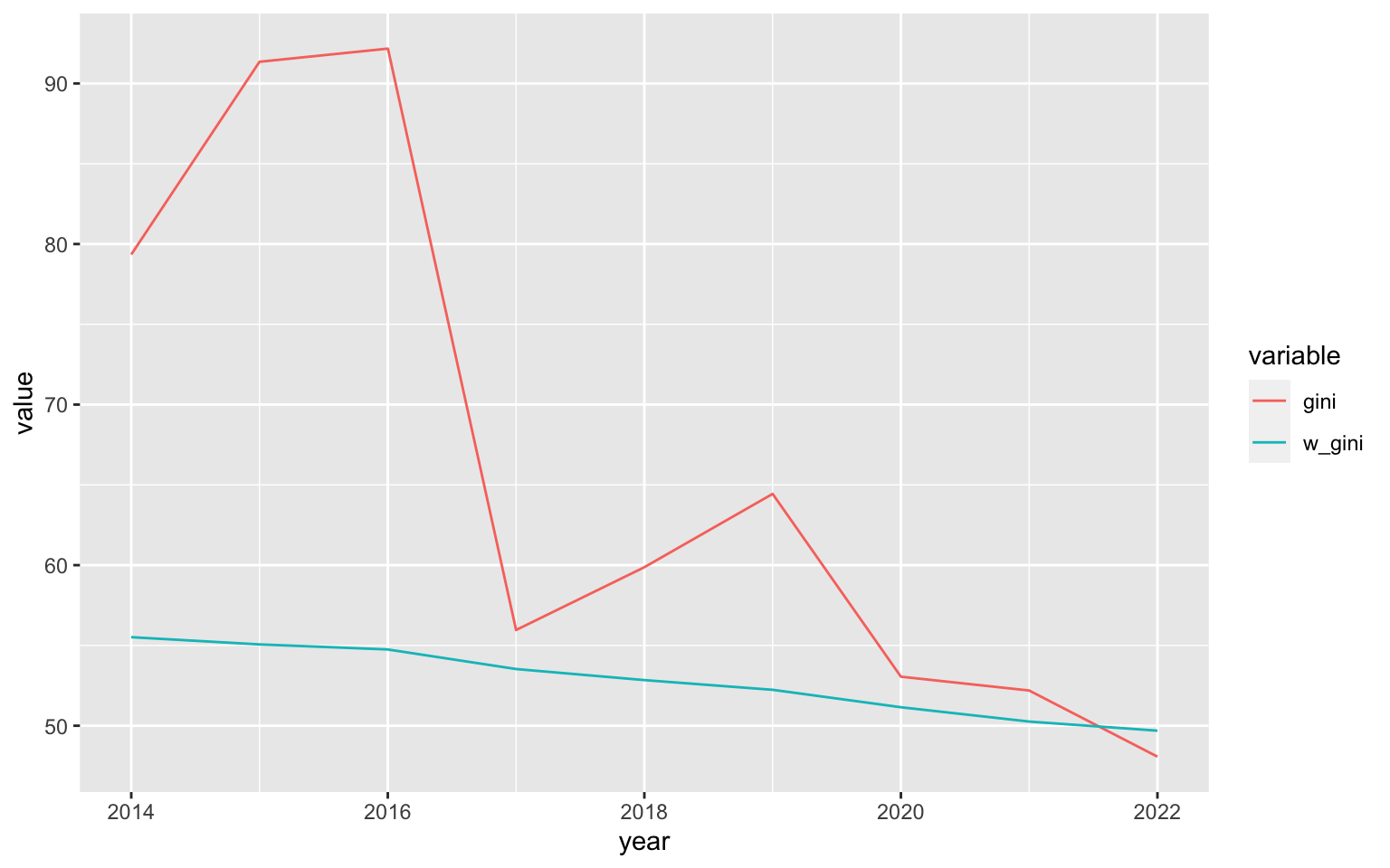

As evident from the plot, the population-weighted GINI is more smooth, which could be due to unpopulated areas exhibiting greater fluctuations in nightlights (such as fires or flares).

A final thing that we can do is calibrate the GINI to an official estimate. I use the africamonitor R API to get World Bank GINI estimates for South Africa.

WB_GINI <- africamonitor::am_data("ZAF", "SI_POV_GINI") %T>% print()
## Key: <Date>
##          Date SI_POV_GINI
##        <Date>       <num>
## 1: 1993-01-01        59.3
## 2: 2000-01-01        57.8
## 3: 2005-01-01        64.8
## 4: 2008-01-01        63.0
## 5: 2010-01-01        63.4
## 6: 2014-01-01        63.0

The last estimate in the series is from 2014, estimating a GINI of 63%. To bring the nightlights data in line with this estimate, I again use optimize() to determine an appropriate power weight:

np_pop_data_pos_14 <- nl_pop_data %>% 
  fsubset(pop > 0 & avg_rad > 0 & year == 2014, year, pop, avg_rad) 

objective <- function(k) {
  nl_gini = np_pop_data_pos_14 %$% w_gini(avg_rad^k, pop) * 100
  abs(63 - nl_gini)
}

res <- optimize(objective, c(0.0001, 5)) %T>% print()
## $minimum
## [1] 1.308973
## 
## $objective
## [1] 0.0002598319

With the ideal weight determined, it is easy to obtain a final calibrated nightlights-based GINI series and use it to extend the World Bank estimate.

final_gini_ts <- nl_pop_data %>% 
  fsubset(pop > 0 & avg_rad > 0) %>%
  fgroup_by(year) %>% 
  fsummarise(nl_gini = w_gini(avg_rad^res$minimum, pop)*100) %T>% print()
##     year  nl_gini
##    <int>    <num>
## 1:  2014 62.99974
## 2:  2015 62.49832
## 3:  2016 62.22387
## 4:  2017 61.22247
## 5:  2018 60.54190
## 6:  2019 59.82656
## 7:  2020 58.83987
## 8:  2021 57.93322
## 9:  2022 57.51001

final_gini_ts %>% 
  merge(WB_GINI %>% fcompute(year = year(Date), wb_gini = SI_POV_GINI), 
        by = "year", all = TRUE) %>% 
  melt("year", na.rm = TRUE) %>% 
  ggplot(aes(x = year, y = value, colour = variable)) + 
      geom_line() + scale_y_continuous(limits = c(50, 70))

It should be noted, at this point, that this estimate and the declining trend it shows may be seriously misguided. Research by Galimberti et al. (2020) using the old DMSP OLS Nightlights series from 1992-2013 for 234 countries and territories, shows that nightlights based inequality measures much better resemble the cross-sectional variation in inequality between countries than the time series dimension within countries.

The example is nevertheless instrumental in showing how the fastverse, in various respects, facilitates and enables complex data science in R.

The Future

Future development of collapse will see an increased use of SIMD instructions to further increase performance. The impact of such instructions - visible in frameworks like Apache arrow and Python’s polars (which is based on arrow) can be considerable. The following shows a benchmark computing the means of a matrix with 100 columns and 1 million rows using base R, collapse 1.9.0 (no SIMD), and collapse 1.9.5 (with SIMD).

library(collapse)
library(microbenchmark)

fmean19 <- collapsedev19::fmean
m <- rnorm(1e8)
dim(m) <- c(1e6, 100) # matrix with 100 columns and 1 million rows

microbenchmark(colMeans(m), 
               fmean19(m, na.rm = FALSE), 
               fmean(m, na.rm = FALSE), 
               fmean(m), # default is na.rm = TRUE, can be changed with set_collapse()
               fmean19(m, nthreads = 4, na.rm = FALSE), 
               fmean(m, nthreads = 4, na.rm = FALSE), 
               fmean(m, nthreads = 4))
## Unit: milliseconds
##                                     expr      min       lq     mean   median       uq       max neval
##                              colMeans(m) 93.09308 97.52766 98.80975 97.99094 99.05563 190.67317   100
##                fmean19(m, na.rm = FALSE) 93.04056 97.47590 97.68101 98.05097 99.14058 100.48612   100
##                  fmean(m, na.rm = FALSE) 12.75202 13.04181 14.05289 13.49043 13.81448  18.79206   100
##                                 fmean(m) 12.67806 13.02974 14.02059 13.49638 13.81009  18.72581   100
##  fmean19(m, nthreads = 4, na.rm = FALSE) 24.84251 25.20573 26.12640 25.52416 27.08612  28.71300   100
##    fmean(m, nthreads = 4, na.rm = FALSE) 13.07941 13.18853 13.96326 13.38853 13.68627  18.04652   100
##                   fmean(m, nthreads = 4) 13.05813 13.18277 13.99704 13.33753 13.71505  19.18242   100

Despite these impressive results, I am somewhat doubtful that much of collapse will benefit from SIMD. The main reason is that SIMD is a low-level vectorization that can be used to speed up simple operations like addition, subtraction, division, and multiplication. This is especially effective with large amounts of adjacent data. But with many groups and little data in each group, serial programming can be just as efficient or even more efficient if it allows writing grouped operations in a non-nested way. So it depends on the data to groups ratio. My arrow benchmark from August 2022 showed just that: with few groups relative to the data size, arrow considerably outperforms collapse and data.table, but with more groups the latter catch up considerably and collapse took lead with many very small groups. More complex statistics algorithms like the median (involving selection) or mode / distinct value count (involving hashing), also cannot (to my knowledge) benefit from SIMD, and here collapse implementations are already pretty much state of the art.

Apart from additional vectorization, I am also considering a possible broadening of the package to support further data manipulation operations such as table joins. This may take a while for me to get into though, so I cannot promise an update including this in 2023. At this stage, I am very happy with the API, so no changes are planned here, and I will also try to keep collapse harmonious with other fastverse packages, in particular data.table and kit.

Most of all, I hope to see an increased breadth of statistical R packages using collapse as a backend, so that its potential for increasing the performance and complexity of statistical R packages is realized in the community. I have in the past assisted package maintainers interested in developing collapse backends and hope to increase further collaborations along these lines.

At last, I wish to thank all users that provided feedback and inspiration or promoted this software in the community, and more generally all people that encouraged, contributed to, and facilitated these projects. Much credit is also due to the CRAN maintainers who endured many of my mistakes and insisted on high standards, which made collapse better and more robust.