Advanced and Fast Data Transformation
collapse-package.Rdcollapse is a C/C++ based package for data transformation and statistical computing in R. Its aims are:
To facilitate complex data transformation, exploration and computing tasks in R.
To help make R code fast, flexible, parsimonious and programmer friendly.
It also implements a class-agnostic approach to data manipulation in R, supporting all major classes.
Getting Started
Read the short vignette on documentation resources, and check out the built-in documentation.
Details
collapse provides an integrated suite of statistical and data manipulation functions that greatly extend and enhance the capabilities of base R. In a nutshell, collapse provides:
Fast C/C++ based (grouped, weighted) computations embedded in highly optimized R code.
More complex statistical, time series / panel data and recursive (list-processing) operations.
A flexible and generic approach supporting and preserving many R objects.
Optimized programming in standard and non-standard evaluation.
The statistical functions in collapse are S3 generic with core methods for vectors, matrices and data frames, and internally support grouped and weighted computations carried out in C/C++.
Functions and core methods seek to preserve object attributes (including column attributes such as variable labels), ensuring flexibility and effective workflows with a very broad range of R objects (including most time-series classes). See the vignette on collapse's handling of R objects.
Missing values are efficiently skipped at C/C++ level. The package default is na.rm = TRUE. This can be changed using set_collapse(na.rm = FALSE). Missing weights are generally supported.
collapse installs with a built-in hierarchical documentation facilitating the use of the package.
The package is coded both in C and C++ and built with Rcpp, but also uses C/C++ functions from data.table, kit, fixest, weights, stats and RcppArmadillo / RcppEigen.
Author(s)
Maintainer: Sebastian Krantz sebastian.krantz@graduateinstitute.ch
Developing / Bug Reporting
Please report issues at https://github.com/SebKrantz/collapse/issues.
Please send pull-requests to the 'development' branch of the repository.
Examples
## Note: this set of examples is is certainly non-exhaustive and does not
## showcase many recent features, but remains a very good starting point
## Let's start with some statistical programming
v <- iris$Sepal.Length
d <- num_vars(iris) # Saving numeric variables
f <- iris$Species # Factor
# Simple statistics
fmean(v) # vector
#> [1] 5.843333
fmean(qM(d)) # matrix (qM is a faster as.matrix)
#> Sepal.Length Sepal.Width Petal.Length Petal.Width
#> 5.843333 3.057333 3.758000 1.199333
fmean(d) # data.frame
#> Sepal.Length Sepal.Width Petal.Length Petal.Width
#> 5.843333 3.057333 3.758000 1.199333
# Preserving data structure
fmean(qM(d), drop = FALSE) # Still a matrix
#> Sepal.Length Sepal.Width Petal.Length Petal.Width
#> [1,] 5.843333 3.057333 3.758 1.199333
fmean(d, drop = FALSE) # Still a data.frame
#> Sepal.Length Sepal.Width Petal.Length Petal.Width
#> 1 5.843333 3.057333 3.758 1.199333
# Weighted statistics, supported by most functions...
w <- abs(rnorm(fnrow(iris)))
fmean(d, w = w)
#> Sepal.Length Sepal.Width Petal.Length Petal.Width
#> 5.812745 3.045097 3.707739 1.172857
# Grouped statistics...
fmean(d, f)
#> Sepal.Length Sepal.Width Petal.Length Petal.Width
#> setosa 5.006 3.428 1.462 0.246
#> versicolor 5.936 2.770 4.260 1.326
#> virginica 6.588 2.974 5.552 2.026
# Groupwise-weighted statistics...
fmean(d, f, w)
#> Sepal.Length Sepal.Width Petal.Length Petal.Width
#> setosa 4.969078 3.383357 1.454456 0.2441565
#> versicolor 5.933818 2.786565 4.220059 1.3122060
#> virginica 6.559617 2.933692 5.533291 1.9895697
# Simple Transformations...
head(fmode(d, TRA = "replace")) # Replacing values with the mode
#> Sepal.Length Sepal.Width Petal.Length Petal.Width
#> 1 5 3 1.5 0.2
#> 2 5 3 1.5 0.2
#> 3 5 3 1.5 0.2
#> 4 5 3 1.5 0.2
#> 5 5 3 1.5 0.2
#> 6 5 3 1.5 0.2
head(fmedian(d, TRA = "-")) # Subtracting the median
#> Sepal.Length Sepal.Width Petal.Length Petal.Width
#> 1 -0.7 0.5 -2.95 -1.1
#> 2 -0.9 0.0 -2.95 -1.1
#> 3 -1.1 0.2 -3.05 -1.1
#> 4 -1.2 0.1 -2.85 -1.1
#> 5 -0.8 0.6 -2.95 -1.1
#> 6 -0.4 0.9 -2.65 -0.9
head(fsum(d, TRA = "%")) # Computing percentages
#> Sepal.Length Sepal.Width Petal.Length Petal.Width
#> 1 0.5818597 0.7631923 0.2483591 0.1111729
#> 2 0.5590416 0.6541648 0.2483591 0.1111729
#> 3 0.5362236 0.6977758 0.2306191 0.1111729
#> 4 0.5248146 0.6759703 0.2660990 0.1111729
#> 5 0.5704507 0.7849978 0.2483591 0.1111729
#> 6 0.6160867 0.8504143 0.3015789 0.2223457
head(fsd(d, TRA = "/")) # Dividing by the standard-deviation (scaling), etc...
#> Sepal.Length Sepal.Width Petal.Length Petal.Width
#> 1 6.158928 8.029986 0.7930671 0.2623854
#> 2 5.917402 6.882845 0.7930671 0.2623854
#> 3 5.675875 7.341701 0.7364195 0.2623854
#> 4 5.555112 7.112273 0.8497148 0.2623854
#> 5 6.038165 8.259414 0.7930671 0.2623854
#> 6 6.521218 8.947698 0.9630101 0.5247707
# Weighted Transformations...
head(fnth(d, 0.75, w = w, TRA = "replace")) # Replacing by the weighted 3rd quartile
#> Sepal.Length Sepal.Width Petal.Length Petal.Width
#> 1 6.4 3.3 5.1 1.8
#> 2 6.4 3.3 5.1 1.8
#> 3 6.4 3.3 5.1 1.8
#> 4 6.4 3.3 5.1 1.8
#> 5 6.4 3.3 5.1 1.8
#> 6 6.4 3.3 5.1 1.8
# Grouped Transformations...
head(fvar(d, f, TRA = "replace")) # Replacing values with the group variance
#> Sepal.Length Sepal.Width Petal.Length Petal.Width
#> 1 0.124249 0.1436898 0.03015918 0.01110612
#> 2 0.124249 0.1436898 0.03015918 0.01110612
#> 3 0.124249 0.1436898 0.03015918 0.01110612
#> 4 0.124249 0.1436898 0.03015918 0.01110612
#> 5 0.124249 0.1436898 0.03015918 0.01110612
#> 6 0.124249 0.1436898 0.03015918 0.01110612
head(fsd(d, f, TRA = "/")) # Grouped scaling
#> Sepal.Length Sepal.Width Petal.Length Petal.Width
#> 1 14.46851 9.233260 8.061544 1.897793
#> 2 13.90112 7.914223 8.061544 1.897793
#> 3 13.33372 8.441838 7.485720 1.897793
#> 4 13.05003 8.178031 8.637369 1.897793
#> 5 14.18481 9.497068 8.061544 1.897793
#> 6 15.31960 10.288490 9.789018 3.795585
head(fmin(d, f, TRA = "-")) # Setting the minimum value in each species to 0
#> Sepal.Length Sepal.Width Petal.Length Petal.Width
#> 1 0.8 1.2 0.4 0.1
#> 2 0.6 0.7 0.4 0.1
#> 3 0.4 0.9 0.3 0.1
#> 4 0.3 0.8 0.5 0.1
#> 5 0.7 1.3 0.4 0.1
#> 6 1.1 1.6 0.7 0.3
head(fsum(d, f, TRA = "/")) # Dividing by the sum (proportions)
#> Sepal.Length Sepal.Width Petal.Length Petal.Width
#> 1 0.02037555 0.02042007 0.01915185 0.01626016
#> 2 0.01957651 0.01750292 0.01915185 0.01626016
#> 3 0.01877747 0.01866978 0.01778386 0.01626016
#> 4 0.01837795 0.01808635 0.02051984 0.01626016
#> 5 0.01997603 0.02100350 0.01915185 0.01626016
#> 6 0.02157411 0.02275379 0.02325581 0.03252033
head(fmedian(d, f, TRA = "-")) # Groupwise de-median
#> Sepal.Length Sepal.Width Petal.Length Petal.Width
#> 1 0.1 0.1 -0.1 0.0
#> 2 -0.1 -0.4 -0.1 0.0
#> 3 -0.3 -0.2 -0.2 0.0
#> 4 -0.4 -0.3 0.0 0.0
#> 5 0.0 0.2 -0.1 0.0
#> 6 0.4 0.5 0.2 0.2
head(ffirst(d, f, TRA = "%%")) # Taking modulus of first group-value, etc. ...
#> Sepal.Length Sepal.Width Petal.Length Petal.Width
#> 1 0.0 0.0 0.0 0
#> 2 4.9 3.0 0.0 0
#> 3 4.7 3.2 1.3 0
#> 4 4.6 3.1 0.1 0
#> 5 5.0 0.1 0.0 0
#> 6 0.3 0.4 0.3 0
# Grouped and weighted transformations...
head(fsd(d, f, w, "/"), 3) # weighted scaling
#> Sepal.Length Sepal.Width Petal.Length Petal.Width
#> 1 13.50637 8.008449 10.004181 1.924217
#> 2 12.97671 6.864385 10.004181 1.924217
#> 3 12.44704 7.322011 9.289596 1.924217
head(fmedian(d, f, w, "-"), 3) # subtracting the weighted group-median
#> Sepal.Length Sepal.Width Petal.Length Petal.Width
#> 1 0.1 0.1 0.0 0
#> 2 -0.1 -0.4 0.0 0
#> 3 -0.3 -0.2 -0.1 0
head(fmode(d, f, w, "replace"), 3) # replace with weighted statistical mode
#> Sepal.Length Sepal.Width Petal.Length Petal.Width
#> 1 5.1 3.4 1.4 0.2
#> 2 5.1 3.4 1.4 0.2
#> 3 5.1 3.4 1.4 0.2
## Some more advanced transformations...
head(fbetween(d)) # Averaging (faster t.: fmean(d, TRA = "replace"))
#> Sepal.Length Sepal.Width Petal.Length Petal.Width
#> 1 5.843333 3.057333 3.758 1.199333
#> 2 5.843333 3.057333 3.758 1.199333
#> 3 5.843333 3.057333 3.758 1.199333
#> 4 5.843333 3.057333 3.758 1.199333
#> 5 5.843333 3.057333 3.758 1.199333
#> 6 5.843333 3.057333 3.758 1.199333
head(fwithin(d)) # Centering (faster than: fmean(d, TRA = "-"))
#> Sepal.Length Sepal.Width Petal.Length Petal.Width
#> 1 -0.7433333 0.44266667 -2.358 -0.9993333
#> 2 -0.9433333 -0.05733333 -2.358 -0.9993333
#> 3 -1.1433333 0.14266667 -2.458 -0.9993333
#> 4 -1.2433333 0.04266667 -2.258 -0.9993333
#> 5 -0.8433333 0.54266667 -2.358 -0.9993333
#> 6 -0.4433333 0.84266667 -2.058 -0.7993333
head(fwithin(d, f, w)) # Grouped and weighted (same as fmean(d, f, w, "-"))
#> Sepal.Length Sepal.Width Petal.Length Petal.Width
#> 1 0.13092175 0.116643 -0.05445601 -0.04415648
#> 2 -0.06907825 -0.383357 -0.05445601 -0.04415648
#> 3 -0.26907825 -0.183357 -0.15445601 -0.04415648
#> 4 -0.36907825 -0.283357 0.04554399 -0.04415648
#> 5 0.03092175 0.216643 -0.05445601 -0.04415648
#> 6 0.43092175 0.516643 0.24554399 0.15584352
head(fwithin(d, f, w, mean = 5)) # Setting a custom mean
#> Sepal.Length Sepal.Width Petal.Length Petal.Width
#> 1 5.130922 5.116643 4.945544 4.955844
#> 2 4.930922 4.616643 4.945544 4.955844
#> 3 4.730922 4.816643 4.845544 4.955844
#> 4 4.630922 4.716643 5.045544 4.955844
#> 5 5.030922 5.216643 4.945544 4.955844
#> 6 5.430922 5.516643 5.245544 5.155844
head(fwithin(d, f, w, theta = 0.76)) # Quasi-centering i.e. d - theta*fbetween(d, f, w)
#> Sepal.Length Sepal.Width Petal.Length Petal.Width
#> 1 1.3235005 0.9286487 0.2946134 0.01444107
#> 2 1.1235005 0.4286487 0.2946134 0.01444107
#> 3 0.9235005 0.6286487 0.1946134 0.01444107
#> 4 0.8235005 0.5286487 0.3946134 0.01444107
#> 5 1.2235005 1.0286487 0.2946134 0.01444107
#> 6 1.6235005 1.3286487 0.5946134 0.21444107
head(fwithin(d, f, w, mean = "overall.mean")) # Preserving the overall mean of the data
#> Sepal.Length Sepal.Width Petal.Length Petal.Width
#> 1 5.943666 3.16174 3.653283 1.128701
#> 2 5.743666 2.66174 3.653283 1.128701
#> 3 5.543666 2.86174 3.553283 1.128701
#> 4 5.443666 2.76174 3.753283 1.128701
#> 5 5.843666 3.26174 3.653283 1.128701
#> 6 6.243666 3.56174 3.953283 1.328701
head(fscale(d)) # Scaling and centering
#> Sepal.Length Sepal.Width Petal.Length Petal.Width
#> 1 -0.8976739 1.01560199 -1.335752 -1.311052
#> 2 -1.1392005 -0.13153881 -1.335752 -1.311052
#> 3 -1.3807271 0.32731751 -1.392399 -1.311052
#> 4 -1.5014904 0.09788935 -1.279104 -1.311052
#> 5 -1.0184372 1.24503015 -1.335752 -1.311052
#> 6 -0.5353840 1.93331463 -1.165809 -1.048667
head(fscale(d, mean = 5, sd = 3)) # Custom scaling and centering
#> Sepal.Length Sepal.Width Petal.Length Petal.Width
#> 1 2.3069784 8.046806 0.9927451 1.066844
#> 2 1.5823985 4.605384 0.9927451 1.066844
#> 3 0.8578187 5.981953 0.8228021 1.066844
#> 4 0.4955288 5.293668 1.1626881 1.066844
#> 5 1.9446885 8.735090 0.9927451 1.066844
#> 6 3.3938481 10.799944 1.5025740 1.854000
head(fscale(d, mean = FALSE, sd = 3)) # Mean preserving scaling
#> Sepal.Length Sepal.Width Petal.Length Petal.Width
#> 1 3.150312 6.104139 -0.24925490 -2.733823
#> 2 2.425732 2.662717 -0.24925490 -2.733823
#> 3 1.701152 4.039286 -0.41919786 -2.733823
#> 4 1.338862 3.351001 -0.07931195 -2.733823
#> 5 2.788022 6.792424 -0.24925490 -2.733823
#> 6 4.237181 8.857277 0.26057397 -1.946667
head(fscale(d, f, w)) # Grouped and weighted scaling and centering
#> Sepal.Length Sepal.Width Petal.Length Petal.Width
#> 1 0.3467210 0.2668941 -0.3891341 -0.4248332
#> 2 -0.1829404 -0.8771700 -0.3891341 -0.4248332
#> 3 -0.7126019 -0.4195444 -1.1037185 -0.4248332
#> 4 -0.9774326 -0.6483572 0.3254502 -0.4248332
#> 5 0.0818903 0.4957070 -0.3891341 -0.4248332
#> 6 1.1412132 1.1821455 1.7546189 1.4993836
head(fscale(d, f, w, mean = 5, sd = 3)) # Custom grouped and weighted scaling and centering
#> Sepal.Length Sepal.Width Petal.Length Petal.Width
#> 1 6.040163 5.800682 3.832598 3.725500
#> 2 4.451179 2.368490 3.832598 3.725500
#> 3 2.862194 3.741367 1.688845 3.725500
#> 4 2.067702 3.054928 5.976351 3.725500
#> 5 5.245671 6.487121 3.832598 3.725500
#> 6 8.423640 8.546436 10.263857 9.498151
head(fscale(d, f, w, mean = FALSE, # Preserving group means
sd = "within.sd")) # and setting group-sd to fsd(fwithin(d, f, w), w = w)
#> Sepal.Length Sepal.Width Petal.Length Petal.Width
#> 1 5.150572 3.482488 1.2890961 0.1615149
#> 2 4.873317 3.057555 1.2890961 0.1615149
#> 3 4.596062 3.227528 0.9854385 0.1615149
#> 4 4.457434 3.142542 1.5927538 0.1615149
#> 5 5.011944 3.567474 1.2890961 0.1615149
#> 6 5.566455 3.822434 2.2000692 0.5358274
head(fscale(d, f, w, mean = "overall.mean", # Full harmonization of group means and variances,
sd = "within.sd")) # while preserving the level and scale of the data.
#> Sepal.Length Sepal.Width Petal.Length Petal.Width
#> 1 5.994238 3.144227 3.542379 1.090216
#> 2 5.716983 2.719295 3.542379 1.090216
#> 3 5.439728 2.889268 3.238722 1.090216
#> 4 5.301100 2.804281 3.846037 1.090216
#> 5 5.855611 3.229214 3.542379 1.090216
#> 6 6.410121 3.484174 4.453352 1.464528
head(get_vars(iris, 1:2)) # Use get_vars for fast selecting, gv is shortcut
#> Sepal.Length Sepal.Width
#> 1 5.1 3.5
#> 2 4.9 3.0
#> 3 4.7 3.2
#> 4 4.6 3.1
#> 5 5.0 3.6
#> 6 5.4 3.9
head(fhdbetween(gv(iris, 1:2), gv(iris, 3:5))) # Linear prediction with factors and covariates
#> Sepal.Length Sepal.Width
#> 1 4.950107 3.389732
#> 2 4.950107 3.389732
#> 3 4.859513 3.374264
#> 4 5.040702 3.405199
#> 5 4.950107 3.389732
#> 6 5.220692 3.560823
head(fhdwithin(gv(iris, 1:2), gv(iris, 3:5))) # Linear partialling out factors and covariates
#> Sepal.Length Sepal.Width
#> 1 0.14989286 0.1102684
#> 2 -0.05010714 -0.3897316
#> 3 -0.15951256 -0.1742640
#> 4 -0.44070173 -0.3051992
#> 5 0.04989286 0.2102684
#> 6 0.17930818 0.3391766
ss(iris, 1:10, 1:2) # Similarly fsubset/ss for fast subsetting rows
#> Sepal.Length Sepal.Width
#> 1 5.1 3.5
#> 2 4.9 3.0
#> 3 4.7 3.2
#> 4 4.6 3.1
#> 5 5.0 3.6
#> 6 5.4 3.9
#> 7 4.6 3.4
#> 8 5.0 3.4
#> 9 4.4 2.9
#> 10 4.9 3.1
# Simple Time-Computations..
head(flag(AirPassengers, -1:3)) # One lead and three lags
#> F1 -- L1 L2 L3
#> Jan 1949 118 112 NA NA NA
#> Feb 1949 132 118 112 NA NA
#> Mar 1949 129 132 118 112 NA
#> Apr 1949 121 129 132 118 112
#> May 1949 135 121 129 132 118
#> Jun 1949 148 135 121 129 132
head(fdiff(EuStockMarkets, # Suitably lagged first and second differences
c(1, frequency(EuStockMarkets)), diff = 1:2))
#> Time Series:
#> Start = c(1991, 130)
#> End = c(1991, 135)
#> Frequency = 260
#> D1.DAX D2.DAX L260D1.DAX L260D2.DAX D1.SMI D2.SMI L260D1.SMI
#> 1991.496 NA NA NA NA NA NA NA
#> 1991.500 -15.12 NA NA NA 10.4 NA NA
#> 1991.504 -7.12 8.00 NA NA -9.9 -20.3 NA
#> 1991.508 14.53 21.65 NA NA 5.5 15.4 NA
#> L260D2.SMI D1.CAC D2.CAC L260D1.CAC L260D2.CAC D1.FTSE D2.FTSE
#> 1991.496 NA NA NA NA NA NA NA
#> 1991.500 NA -22.3 NA NA NA 16.6 NA
#> 1991.504 NA -32.5 -10.2 NA NA -12.0 -28.6
#> 1991.508 NA -9.9 22.6 NA NA 22.2 34.2
#> L260D1.FTSE L260D2.FTSE
#> 1991.496 NA NA
#> 1991.500 NA NA
#> 1991.504 NA NA
#> 1991.508 NA NA
#> [ reached 'max' / getOption("max.print") -- omitted 2 rows ]
head(fdiff(EuStockMarkets, rho = 0.87)) # Quasi-differences (x_t - rho*x_t-1)
#> Time Series:
#> Start = c(1991, 130)
#> End = c(1991, 135)
#> Frequency = 260
#> DAX SMI CAC FTSE
#> 1991.496 NA NA NA NA
#> 1991.500 196.6175 228.553 208.164 334.268
#> 1991.504 202.6519 209.605 195.065 307.826
#> 1991.508 223.3763 223.718 213.440 340.466
#> 1991.512 207.8552 221.433 237.053 335.452
#> 1991.515 202.8108 204.258 215.203 305.111
head(fdiff(EuStockMarkets, log = TRUE)) # Log-differences
#> Time Series:
#> Start = c(1991, 130)
#> End = c(1991, 135)
#> Frequency = 260
#> DAX SMI CAC FTSE
#> 1991.496 NA NA NA NA
#> 1991.500 -0.009326550 0.006178360 -0.012658756 0.006770286
#> 1991.504 -0.004422175 -0.005880448 -0.018740638 -0.004889587
#> 1991.508 0.009003794 0.003271184 -0.005779182 0.009027020
#> 1991.512 -0.001778217 0.001483372 0.008743353 0.005771847
#> 1991.515 -0.004676712 -0.008933417 -0.005120160 -0.007230164
head(fgrowth(EuStockMarkets)) # Exact growth rates (percentage change)
#> Time Series:
#> Start = c(1991, 130)
#> End = c(1991, 135)
#> Frequency = 260
#> DAX SMI CAC FTSE
#> 1991.496 NA NA NA NA
#> 1991.500 -0.9283193 0.6197485 -1.2578971 0.6793256
#> 1991.504 -0.4412412 -0.5863192 -1.8566124 -0.4877652
#> 1991.508 0.9044450 0.3276540 -0.5762515 0.9067887
#> 1991.512 -0.1776637 0.1484472 0.8781687 0.5788536
#> 1991.515 -0.4665793 -0.8893632 -0.5107074 -0.7204089
head(fgrowth(EuStockMarkets, logdiff = TRUE)) # Log-difference growth rates (percentage change)
#> Time Series:
#> Start = c(1991, 130)
#> End = c(1991, 135)
#> Frequency = 260
#> DAX SMI CAC FTSE
#> 1991.496 NA NA NA NA
#> 1991.500 -0.9326550 0.6178360 -1.2658756 0.6770286
#> 1991.504 -0.4422175 -0.5880448 -1.8740638 -0.4889587
#> 1991.508 0.9003794 0.3271184 -0.5779182 0.9027020
#> 1991.512 -0.1778217 0.1483372 0.8743353 0.5771847
#> 1991.515 -0.4676712 -0.8933417 -0.5120160 -0.7230164
# Note that it is not necessary to use factors for grouping.
fmean(gv(mtcars, -c(2,8:9)), mtcars$cyl) # Can also use vector (internally converted using qF())
#> mpg disp hp drat wt qsec gear carb
#> 4 26.66364 105.1364 82.63636 4.070909 2.285727 19.13727 4.090909 1.545455
#> 6 19.74286 183.3143 122.28571 3.585714 3.117143 17.97714 3.857143 3.428571
#> 8 15.10000 353.1000 209.21429 3.229286 3.999214 16.77214 3.285714 3.500000
fmean(gv(mtcars, -c(2,8:9)),
gv(mtcars, c(2,8:9))) # or a list of vector (internally grouped using GRP())
#> mpg disp hp drat wt qsec gear carb
#> 4.0.1 26.00000 120.3000 91.00000 4.430000 2.140000 16.70000 5.000000 2.000000
#> 4.1.0 22.90000 135.8667 84.66667 3.770000 2.935000 20.97000 3.666667 1.666667
#> 4.1.1 28.37143 89.8000 80.57143 4.148571 2.028286 18.70000 4.142857 1.428571
#> 6.0.1 20.56667 155.0000 131.66667 3.806667 2.755000 16.32667 4.333333 4.666667
#> 6.1.0 19.12500 204.5500 115.25000 3.420000 3.388750 19.21500 3.500000 2.500000
#> 8.0.0 15.05000 357.6167 194.16667 3.120833 4.104083 17.14250 3.000000 3.083333
#> 8.0.1 15.40000 326.0000 299.50000 3.880000 3.370000 14.55000 5.000000 6.000000
g <- GRP(mtcars, ~ cyl + vs + am) # It is also possible to create grouping objects
print(g) # These are instructive to learn about the grouping,
#> collapse grouping object of length 32 with 7 ordered groups
#>
#> Call: GRP.default(X = mtcars, by = ~cyl + vs + am), X is unsorted
#>
#> Distribution of group sizes:
#> Min. 1st Qu. Median Mean 3rd Qu. Max.
#> 1.000 2.500 3.000 4.571 5.500 12.000
#>
#> Groups with sizes:
#> 4.0.1 4.1.0 4.1.1 6.0.1 6.1.0 8.0.0 8.0.1
#> 1 3 7 3 4 12 2
plot(g) # and are directly handed down to C++ code
 fmean(gv(mtcars, -c(2,8:9)), g) # This can speed up multiple computations over same groups
#> mpg disp hp drat wt qsec gear carb
#> 4.0.1 26.00000 120.3000 91.00000 4.430000 2.140000 16.70000 5.000000 2.000000
#> 4.1.0 22.90000 135.8667 84.66667 3.770000 2.935000 20.97000 3.666667 1.666667
#> 4.1.1 28.37143 89.8000 80.57143 4.148571 2.028286 18.70000 4.142857 1.428571
#> 6.0.1 20.56667 155.0000 131.66667 3.806667 2.755000 16.32667 4.333333 4.666667
#> 6.1.0 19.12500 204.5500 115.25000 3.420000 3.388750 19.21500 3.500000 2.500000
#> 8.0.0 15.05000 357.6167 194.16667 3.120833 4.104083 17.14250 3.000000 3.083333
#> 8.0.1 15.40000 326.0000 299.50000 3.880000 3.370000 14.55000 5.000000 6.000000
fsd(gv(mtcars, -c(2,8:9)), g)
#> mpg disp hp drat wt qsec gear
#> 4.0.1 NA NA NA NA NA NA NA
#> 4.1.0 1.4525839 13.969371 19.65536 0.1300000 0.4075230 1.67143651 0.5773503
#> 4.1.1 4.7577005 18.802128 24.14441 0.3783926 0.4400840 0.94546285 0.3779645
#> 6.0.1 0.7505553 8.660254 37.52777 0.1616581 0.1281601 0.76872188 0.5773503
#> 6.1.0 1.6317169 44.742634 9.17878 0.5919459 0.1162164 0.81590441 0.5773503
#> 8.0.0 2.7743959 71.823494 33.35984 0.2302749 0.7683069 0.80164745 0.0000000
#> 8.0.1 0.5656854 35.355339 50.20458 0.4808326 0.2828427 0.07071068 0.0000000
#> carb
#> 4.0.1 NA
#> 4.1.0 0.5773503
#> 4.1.1 0.5345225
#> 6.0.1 1.1547005
#> 6.1.0 1.7320508
#> 8.0.0 0.9003366
#> 8.0.1 2.8284271
# Factors can efficiently be created using qF()
f1 <- qF(mtcars$cyl) # Unlike GRP objects, factors are checked for NA's
f2 <- qF(mtcars$cyl, na.exclude = FALSE) # This can however be avoided through this option
class(f2) # Note the added class
#> [1] "factor" "na.included"
library(microbenchmark)
microbenchmark(fmean(mtcars, f1), fmean(mtcars, f2)) # A minor difference, larger on larger data
#> Unit: microseconds
#> expr min lq mean median uq max neval
#> fmean(mtcars, f1) 4.264 4.551 5.03767 4.715 4.9405 22.263 100
#> fmean(mtcars, f2) 4.059 4.346 5.24964 4.510 4.6535 65.887 100
with(mtcars, finteraction(cyl, vs, am)) # Efficient interactions of vectors and/or factors
#> [1] 6.0.1 6.0.1 4.1.1 6.1.0 8.0.0 6.1.0 8.0.0 4.1.0 4.1.0 6.1.0 6.1.0 8.0.0
#> [13] 8.0.0 8.0.0 8.0.0 8.0.0 8.0.0 4.1.1 4.1.1 4.1.1 4.1.0 8.0.0 8.0.0 8.0.0
#> [25] 8.0.0 4.1.1 4.0.1 4.1.1 8.0.1 6.0.1 8.0.1 4.1.1
#> Levels: 4.0.1 4.1.0 4.1.1 6.0.1 6.1.0 8.0.0 8.0.1
finteraction(gv(mtcars, c(2,8:9))) # .. or lists of vectors/factors
#> [1] 6.0.1 6.0.1 4.1.1 6.1.0 8.0.0 6.1.0 8.0.0 4.1.0 4.1.0 6.1.0 6.1.0 8.0.0
#> [13] 8.0.0 8.0.0 8.0.0 8.0.0 8.0.0 4.1.1 4.1.1 4.1.1 4.1.0 8.0.0 8.0.0 8.0.0
#> [25] 8.0.0 4.1.1 4.0.1 4.1.1 8.0.1 6.0.1 8.0.1 4.1.1
#> Levels: 4.0.1 4.1.0 4.1.1 6.0.1 6.1.0 8.0.0 8.0.1
# Simple row- or column-wise computations on matrices or data frames with dapply()
dapply(mtcars, quantile) # column quantiles
#> mpg cyl disp hp drat wt qsec vs am gear carb
#> 0% 10.400 4 71.100 52.0 2.760 1.51300 14.5000 0 0 3 1
#> 25% 15.425 4 120.825 96.5 3.080 2.58125 16.8925 0 0 3 2
#> 50% 19.200 6 196.300 123.0 3.695 3.32500 17.7100 0 0 4 2
#> 75% 22.800 8 326.000 180.0 3.920 3.61000 18.9000 1 1 4 4
#> 100% 33.900 8 472.000 335.0 4.930 5.42400 22.9000 1 1 5 8
dapply(mtcars, quantile, MARGIN = 1) # Row-quantiles
#> 0% 25% 50% 75% 100%
#> Mazda RX4 0 3.2600 4.000 18.730 160.0
#> Mazda RX4 Wag 0 3.3875 4.000 19.010 160.0
#> Datsun 710 1 1.6600 4.000 20.705 108.0
#> Hornet 4 Drive 0 2.0000 3.215 20.420 258.0
#> Hornet Sportabout 0 2.5000 3.440 17.860 360.0
#> Valiant 0 1.8800 3.460 19.160 225.0
#> Duster 360 0 3.1050 4.000 15.070 360.0
#> Merc 240D 0 2.5950 4.000 22.200 146.7
#> Merc 230 0 2.5750 4.000 22.850 140.8
#> Merc 280 0 3.6800 4.000 18.750 167.6
#> Merc 280C 0 3.6800 4.000 18.350 167.6
#> Merc 450SE 0 3.0000 4.070 16.900 275.8
#> Merc 450SL 0 3.0000 3.730 17.450 275.8
#> Merc 450SLC 0 3.0000 3.780 16.600 275.8
#> [ reached 'max' / getOption("max.print") -- omitted 18 rows ]
# dapply preserves the data structure of any matrices / data frames passed
# Some fast matrix row/column functions are also provided by the matrixStats package
# Similarly, BY performs grouped comptations
BY(mtcars, f2, quantile)
#> mpg cyl disp hp drat wt qsec vs am gear carb
#> 4.0% 21.4 4 71.10 52.0 3.690 1.5130 16.70 0 0.0 3 1
#> 4.25% 22.8 4 78.85 65.5 3.810 1.8850 18.56 1 0.5 4 1
#> 4.50% 26.0 4 108.00 91.0 4.080 2.2000 18.90 1 1.0 4 2
#> 4.75% 30.4 4 120.65 96.0 4.165 2.6225 19.95 1 1.0 4 2
#> 4.100% 33.9 4 146.70 113.0 4.930 3.1900 22.90 1 1.0 5 2
#> 6.0% 17.8 6 145.00 105.0 2.760 2.6200 15.50 0 0.0 3 1
#> [ reached 'max' / getOption("max.print") -- omitted 9 rows ]
BY(mtcars, f2, quantile, expand.wide = TRUE)
#> mpg.0% mpg.25% mpg.50% mpg.75% mpg.100% cyl.0% cyl.25% cyl.50% cyl.75%
#> 4 21.4 22.8 26 30.4 33.9 4 4 4 4
#> cyl.100% disp.0% disp.25% disp.50% disp.75% disp.100% hp.0% hp.25% hp.50%
#> 4 4 71.1 78.85 108 120.65 146.7 52 65.5 91
#> hp.75% hp.100% drat.0% drat.25% drat.50% drat.75% drat.100% wt.0% wt.25%
#> 4 96 113 3.69 3.81 4.08 4.165 4.93 1.513 1.885
#> wt.50% wt.75% wt.100% qsec.0% qsec.25% qsec.50% qsec.75% qsec.100% vs.0%
#> 4 2.2 2.6225 3.19 16.7 18.56 18.9 19.95 22.9 0
#> vs.25% vs.50% vs.75% vs.100% am.0% am.25% am.50% am.75% am.100% gear.0%
#> 4 1 1 1 1 0 0.5 1 1 1 3
#> gear.25% gear.50% gear.75% gear.100% carb.0% carb.25% carb.50% carb.75%
#> 4 4 4 4 5 1 1 2 2
#> carb.100%
#> 4 2
#> [ reached 'max' / getOption("max.print") -- omitted 2 rows ]
# For efficient (grouped) replacing and sweeping out computed statistics, use TRA()
sds <- fsd(mtcars)
head(TRA(mtcars, sds, "/")) # Simple scaling (if sd's not needed, use fsd(mtcars, TRA = "/"))
#> mpg cyl disp hp drat wt
#> Mazda RX4 3.484351 3.35961 1.2909608 1.604367 7.294100 2.677684
#> Mazda RX4 Wag 3.484351 3.35961 1.2909608 1.604367 7.294100 2.938298
#> Datsun 710 3.783009 2.23974 0.8713986 1.356419 7.200586 2.371079
#> Hornet 4 Drive 3.550719 3.35961 2.0816744 1.604367 5.760468 3.285784
#> Hornet Sportabout 3.102731 4.47948 2.9046619 2.552402 5.891388 3.515738
#> Valiant 3.003178 3.35961 1.8154137 1.531441 5.161978 3.536178
#> qsec vs am gear carb
#> Mazda RX4 9.211261 0.000000 2.004044 5.421494 2.4764735
#> Mazda RX4 Wag 9.524645 0.000000 2.004044 5.421494 2.4764735
#> Datsun 710 10.414433 1.984063 2.004044 5.421494 0.6191184
#> Hornet 4 Drive 10.878913 1.984063 0.000000 4.066120 0.6191184
#> Hornet Sportabout 9.524645 0.000000 0.000000 4.066120 1.2382368
#> Valiant 11.315413 1.984063 0.000000 4.066120 0.6191184
microbenchmark(TRA(mtcars, sds, "/"), sweep(mtcars, 2, sds, "/")) # A remarkable performance gain..
#> Unit: microseconds
#> expr min lq mean median uq
#> TRA(mtcars, sds, "/") 2.378 3.1980 18.84319 6.4985 15.2725
#> sweep(mtcars, 2, sds, "/") 350.714 421.5005 1041.08102 714.3840 1405.1930
#> max neval
#> 652.146 100
#> 5053.865 100
sds <- fsd(mtcars, f2)
head(TRA(mtcars, sds, "/", f2)) # Groupd scaling (if sd's not needed: fsd(mtcars, f2, TRA = "/"))
#> mpg cyl disp hp drat wt qsec
#> Mazda RX4 14.447218 Inf 3.849628 4.534121 8.192327 7.352414 9.643407
#> Mazda RX4 Wag 14.447218 Inf 3.849628 4.534121 8.192327 8.068012 9.971493
#> Datsun 710 5.055626 Inf 4.019114 4.442421 10.534350 4.073293 11.061282
#> Hornet 4 Drive 14.722403 Inf 6.207525 4.534121 6.469838 9.022142 11.389297
#> Hornet Sportabout 7.304550 Inf 5.311981 3.432928 8.459515 4.529864 14.230606
#> Valiant 12.452126 Inf 5.413539 4.328025 5.797647 9.709677 11.846275
#> vs am gear carb
#> Mazda RX4 0.000000 1.870829 5.796551 2.2067091
#> Mazda RX4 Wag 0.000000 1.870829 5.796551 2.2067091
#> Datsun 710 3.316625 2.140872 7.416198 1.9148542
#> Hornet 4 Drive 1.870829 0.000000 4.347413 0.5516773
#> Hornet Sportabout NaN 0.000000 4.130678 1.2848321
#> Valiant 1.870829 0.000000 4.347413 0.5516773
# All functions above perserve the structure of matrices / data frames
# If conversions are required, use these efficient functions:
mtcarsM <- qM(mtcars) # Matrix from data.frame
head(qDF(mtcarsM)) # data.frame from matrix columns
#> mpg cyl disp hp drat wt qsec vs am gear carb
#> Mazda RX4 21.0 6 160 110 3.90 2.620 16.46 0 1 4 4
#> Mazda RX4 Wag 21.0 6 160 110 3.90 2.875 17.02 0 1 4 4
#> Datsun 710 22.8 4 108 93 3.85 2.320 18.61 1 1 4 1
#> Hornet 4 Drive 21.4 6 258 110 3.08 3.215 19.44 1 0 3 1
#> Hornet Sportabout 18.7 8 360 175 3.15 3.440 17.02 0 0 3 2
#> Valiant 18.1 6 225 105 2.76 3.460 20.22 1 0 3 1
head(mrtl(mtcarsM, TRUE, "data.frame")) # data.frame from matrix rows, etc..
#> Mazda RX4 Mazda RX4 Wag Datsun 710 Hornet 4 Drive Hornet Sportabout Valiant
#> mpg 21 21 22.8 21.4 18.7 18.1
#> cyl 6 6 4.0 6.0 8.0 6.0
#> Duster 360 Merc 240D Merc 230 Merc 280 Merc 280C Merc 450SE Merc 450SL
#> mpg 14.3 24.4 22.8 19.2 17.8 16.4 17.3
#> cyl 8.0 4.0 4.0 6.0 6.0 8.0 8.0
#> Merc 450SLC Cadillac Fleetwood Lincoln Continental Chrysler Imperial
#> mpg 15.2 10.4 10.4 14.7
#> cyl 8.0 8.0 8.0 8.0
#> Fiat 128 Honda Civic Toyota Corolla Toyota Corona Dodge Challenger
#> mpg 32.4 30.4 33.9 21.5 15.5
#> cyl 4.0 4.0 4.0 4.0 8.0
#> AMC Javelin Camaro Z28 Pontiac Firebird Fiat X1-9 Porsche 914-2
#> mpg 15.2 13.3 19.2 27.3 26
#> cyl 8.0 8.0 8.0 4.0 4
#> Lotus Europa Ford Pantera L Ferrari Dino Maserati Bora Volvo 142E
#> mpg 30.4 15.8 19.7 15 21.4
#> cyl 4.0 8.0 6.0 8 4.0
#> [ reached 'max' / getOption("max.print") -- omitted 4 rows ]
head(qDT(mtcarsM, "cars")) # Saving row.names when converting matrix to data.table
#> cars mpg cyl disp hp drat wt qsec vs am
#> <char> <num> <num> <num> <num> <num> <num> <num> <num> <num>
#> 1: Mazda RX4 21.0 6 160 110 3.90 2.620 16.46 0 1
#> 2: Mazda RX4 Wag 21.0 6 160 110 3.90 2.875 17.02 0 1
#> 3: Datsun 710 22.8 4 108 93 3.85 2.320 18.61 1 1
#> 4: Hornet 4 Drive 21.4 6 258 110 3.08 3.215 19.44 1 0
#> gear carb
#> <num> <num>
#> 1: 4 4
#> 2: 4 4
#> 3: 4 1
#> 4: 3 1
#> [ reached 'max' / getOption("max.print") -- omitted 2 rows ]
head(qDT(mtcars, "cars")) # Same use a data.frame
#> cars mpg cyl disp hp drat wt qsec vs am
#> <char> <num> <num> <num> <num> <num> <num> <num> <num> <num>
#> 1: Mazda RX4 21.0 6 160 110 3.90 2.620 16.46 0 1
#> 2: Mazda RX4 Wag 21.0 6 160 110 3.90 2.875 17.02 0 1
#> 3: Datsun 710 22.8 4 108 93 3.85 2.320 18.61 1 1
#> 4: Hornet 4 Drive 21.4 6 258 110 3.08 3.215 19.44 1 0
#> gear carb
#> <num> <num>
#> 1: 4 4
#> 2: 4 4
#> 3: 4 1
#> 4: 3 1
#> [ reached 'max' / getOption("max.print") -- omitted 2 rows ]
## Now let's get some real data and see how we can use this power for data manipulation
head(wlddev) # World Bank World Development Data: 216 countries, 61 years, 5 series (columns 9-13)
#> country iso3c date year decade region income OECD PCGDP
#> 1 Afghanistan AFG 1961-01-01 1960 1960 South Asia Low income FALSE NA
#> 2 Afghanistan AFG 1962-01-01 1961 1960 South Asia Low income FALSE NA
#> 3 Afghanistan AFG 1963-01-01 1962 1960 South Asia Low income FALSE NA
#> 4 Afghanistan AFG 1964-01-01 1963 1960 South Asia Low income FALSE NA
#> 5 Afghanistan AFG 1965-01-01 1964 1960 South Asia Low income FALSE NA
#> LIFEEX GINI ODA POP
#> 1 32.446 NA 116769997 8996973
#> 2 32.962 NA 232080002 9169410
#> 3 33.471 NA 112839996 9351441
#> 4 33.971 NA 237720001 9543205
#> 5 34.463 NA 295920013 9744781
#> [ reached 'max' / getOption("max.print") -- omitted 1 rows ]
# Starting with some discriptive tools...
namlab(wlddev, class = TRUE) # Show variable names, labels and classes
#> Variable Class
#> 1 country character
#> 2 iso3c factor
#> 3 date Date
#> 4 year integer
#> 5 decade integer
#> 6 region factor
#> 7 income factor
#> 8 OECD logical
#> 9 PCGDP numeric
#> 10 LIFEEX numeric
#> 11 GINI numeric
#> 12 ODA numeric
#> 13 POP numeric
#> Label
#> 1 Country Name
#> 2 Country Code
#> 3 Date Recorded (Fictitious)
#> 4 Year
#> 5 Decade
#> 6 Region
#> 7 Income Level
#> 8 Is OECD Member Country?
#> 9 GDP per capita (constant 2010 US$)
#> 10 Life expectancy at birth, total (years)
#> 11 Gini index (World Bank estimate)
#> 12 Net official development assistance and official aid received (constant 2018 US$)
#> 13 Population, total
fnobs(wlddev) # Observation count
#> country iso3c date year decade region income OECD PCGDP LIFEEX
#> 13176 13176 13176 13176 13176 13176 13176 13176 9470 11670
#> GINI ODA POP
#> 1744 8608 12919
pwnobs(wlddev) # Pairwise observation count
#> country iso3c date year decade region income OECD PCGDP LIFEEX GINI
#> country 13176 13176 13176 13176 13176 13176 13176 13176 9470 11670 1744
#> iso3c 13176 13176 13176 13176 13176 13176 13176 13176 9470 11670 1744
#> date 13176 13176 13176 13176 13176 13176 13176 13176 9470 11670 1744
#> year 13176 13176 13176 13176 13176 13176 13176 13176 9470 11670 1744
#> decade 13176 13176 13176 13176 13176 13176 13176 13176 9470 11670 1744
#> ODA POP
#> country 8608 12919
#> iso3c 8608 12919
#> date 8608 12919
#> year 8608 12919
#> decade 8608 12919
#> [ reached 'max' / getOption("max.print") -- omitted 8 rows ]
head(fnobs(wlddev, wlddev$country)) # Grouped observation count
#> country iso3c date year decade region income OECD PCGDP LIFEEX
#> Afghanistan 61 61 61 61 61 61 61 61 18 60
#> Albania 61 61 61 61 61 61 61 61 40 60
#> Algeria 61 61 61 61 61 61 61 61 60 60
#> American Samoa 61 61 61 61 61 61 61 61 17 0
#> Andorra 61 61 61 61 61 61 61 61 50 0
#> GINI ODA POP
#> Afghanistan 0 60 60
#> Albania 9 32 60
#> Algeria 3 60 60
#> American Samoa 0 0 60
#> Andorra 0 0 60
#> [ reached 'max' / getOption("max.print") -- omitted 1 rows ]
fndistinct(wlddev) # Distinct values
#> country iso3c date year decade region income OECD PCGDP LIFEEX
#> 216 216 61 61 7 7 4 2 9470 10548
#> GINI ODA POP
#> 368 7832 12877
descr(wlddev) # Describe data
#> Dataset: wlddev, 13 Variables, N = 13176
#> --------------------------------------------------------------------------------
#> country (character): Country Name
#> Statistics
#> N Ndist
#> 13176 216
#> Table
#> Freq Perc
#> Afghanistan 61 0.46
#> Albania 61 0.46
#> Algeria 61 0.46
#> American Samoa 61 0.46
#> Andorra 61 0.46
#> Angola 61 0.46
#> Antigua and Barbuda 61 0.46
#> Argentina 61 0.46
#> Armenia 61 0.46
#> Aruba 61 0.46
#> Australia 61 0.46
#> Austria 61 0.46
#> Azerbaijan 61 0.46
#> Bahamas, The 61 0.46
#> ... 202 Others 12322 93.52
#>
#> Summary of Table Frequencies
#> Min. 1st Qu. Median Mean 3rd Qu. Max.
#> 61 61 61 61 61 61
#> --------------------------------------------------------------------------------
#> iso3c (factor): Country Code
#> Statistics
#> N Ndist
#> 13176 216
#> Table
#> Freq Perc
#> ABW 61 0.46
#> AFG 61 0.46
#> AGO 61 0.46
#> ALB 61 0.46
#> AND 61 0.46
#> ARE 61 0.46
#> ARG 61 0.46
#> ARM 61 0.46
#> ASM 61 0.46
#> ATG 61 0.46
#> AUS 61 0.46
#> AUT 61 0.46
#> AZE 61 0.46
#> BDI 61 0.46
#> ... 202 Others 12322 93.52
#>
#> Summary of Table Frequencies
#> Min. 1st Qu. Median Mean 3rd Qu. Max.
#> 61 61 61 61 61 61
#> --------------------------------------------------------------------------------
#> date (Date): Date Recorded (Fictitious)
#> Statistics
#> N Ndist Min Max
#> 13176 61 1961-01-01 2021-01-01
#> --------------------------------------------------------------------------------
#> year (integer): Year
#> Statistics
#> N Ndist Mean SD Min Max Skew Kurt
#> 13176 61 1990 17.61 1960 2020 -0 1.8
#> Quantiles
#> 1% 5% 10% 25% 50% 75% 90% 95% 99%
#> 1960 1963 1966 1975 1990 2005 2014 2017 2020
#> --------------------------------------------------------------------------------
#> decade (integer): Decade
#> Statistics
#> N Ndist Mean SD Min Max Skew Kurt
#> 13176 7 1985.57 17.51 1960 2020 0.03 1.79
#> Quantiles
#> 1% 5% 10% 25% 50% 75% 90% 95% 99%
#> 1960 1960 1960 1970 1990 2000 2010 2010 2020
#> --------------------------------------------------------------------------------
#> region (factor): Region
#> Statistics
#> N Ndist
#> 13176 7
#> Table
#> Freq Perc
#> Europe & Central Asia 3538 26.85
#> Sub-Saharan Africa 2928 22.22
#> Latin America & Caribbean 2562 19.44
#> East Asia & Pacific 2196 16.67
#> Middle East & North Africa 1281 9.72
#> South Asia 488 3.70
#> North America 183 1.39
#> --------------------------------------------------------------------------------
#> income (factor): Income Level
#> Statistics
#> N Ndist
#> 13176 4
#> Table
#> Freq Perc
#> High income 4819 36.57
#> Upper middle income 3660 27.78
#> Lower middle income 2867 21.76
#> Low income 1830 13.89
#> --------------------------------------------------------------------------------
#> OECD (logical): Is OECD Member Country?
#> Statistics
#> N Ndist
#> 13176 2
#> Table
#> Freq Perc
#> FALSE 10980 83.33
#> TRUE 2196 16.67
#> --------------------------------------------------------------------------------
#> PCGDP (numeric): GDP per capita (constant 2010 US$)
#> Statistics (28.13% NAs)
#> N Ndist Mean SD Min Max Skew Kurt
#> 9470 9470 12048.78 19077.64 132.08 196061.42 3.13 17.12
#> Quantiles
#> 1% 5% 10% 25% 50% 75% 90% 95%
#> 227.71 399.62 555.55 1303.19 3767.16 14787.03 35646.02 48507.84
#> 99%
#> 92340.28
#> --------------------------------------------------------------------------------
#> LIFEEX (numeric): Life expectancy at birth, total (years)
#> Statistics (11.43% NAs)
#> N Ndist Mean SD Min Max Skew Kurt
#> 11670 10548 64.3 11.48 18.91 85.42 -0.67 2.67
#> Quantiles
#> 1% 5% 10% 25% 50% 75% 90% 95% 99%
#> 35.83 42.77 46.83 56.36 67.44 72.95 77.08 79.34 82.36
#> --------------------------------------------------------------------------------
#> GINI (numeric): Gini index (World Bank estimate)
#> Statistics (86.76% NAs)
#> N Ndist Mean SD Min Max Skew Kurt
#> 1744 368 38.53 9.2 20.7 65.8 0.6 2.53
#> Quantiles
#> 1% 5% 10% 25% 50% 75% 90% 95% 99%
#> 24.6 26.3 27.6 31.5 36.4 45 52.6 55.98 60.5
#> --------------------------------------------------------------------------------
#> ODA (numeric): Net official development assistance and official aid received (constant 2018 US$)
#> Statistics (34.67% NAs)
#> N Ndist Mean SD Min Max Skew
#> 8608 7832 454'720131 868'712654 -997'679993 2.56715605e+10 6.98
#> Kurt
#> 114.89
#> Quantiles
#> 1% 5% 10% 25% 50% 75%
#> -12'593999.7 1'363500.01 8'347000.31 44'887499.8 165'970001 495'042503
#> 90% 95% 99%
#> 1.18400697e+09 1.93281696e+09 3.73380782e+09
#> --------------------------------------------------------------------------------
#> POP (numeric): Population, total
#> Statistics (1.95% NAs)
#> N Ndist Mean SD Min Max Skew Kurt
#> 12919 12877 24'245971.6 102'120674 2833 1.39771500e+09 9.75 108.91
#> Quantiles
#> 1% 5% 10% 25% 50% 75% 90%
#> 8698.84 31083.3 62268.4 443791 4'072517 12'816178 46'637331.4
#> 95% 99%
#> 81'177252.5 308'862641
#> --------------------------------------------------------------------------------
varying(wlddev, ~ country) # Show which variables vary within countries
#> iso3c date year decade region income OECD PCGDP LIFEEX GINI ODA
#> FALSE TRUE TRUE TRUE FALSE FALSE FALSE TRUE TRUE TRUE TRUE
#> POP
#> TRUE
qsu(wlddev, pid = ~ country, # Panel-summarize columns 9 though 12 of this data
cols = 9:12, vlabels = TRUE) # (between and within countries)
#> , , PCGDP: GDP per capita (constant 2010 US$)
#>
#> N/T Mean SD Min Max
#> Overall 9470 12048.778 19077.6416 132.0776 196061.417
#> Between 206 12962.6054 20189.9007 253.1886 141200.38
#> Within 45.9709 12048.778 6723.6808 -33504.8721 76767.5254
#>
#> , , LIFEEX: Life expectancy at birth, total (years)
#>
#> N/T Mean SD Min Max
#> Overall 11670 64.2963 11.4764 18.907 85.4171
#> Between 207 64.9537 9.8936 40.9663 85.4171
#> Within 56.3768 64.2963 6.0842 32.9068 84.4198
#>
#> , , GINI: Gini index (World Bank estimate)
#>
#> N/T Mean SD Min Max
#> Overall 1744 38.5341 9.2006 20.7 65.8
#> Between 167 39.4233 8.1356 24.8667 61.7143
#> Within 10.4431 38.5341 2.9277 25.3917 55.3591
#>
#> , , ODA: Net official development assistance and official aid received (constant 2018 US$)
#>
#> N/T Mean SD Min Max
#> Overall 8608 454'720131 868'712654 -997'679993 2.56715605e+10
#> Between 178 439'168412 569'049959 468717.916 3.62337432e+09
#> Within 48.3596 454'720131 650'709624 -2.44379420e+09 2.45610972e+10
#>
qsu(wlddev, ~ region, ~ country, # Do all of that by region and also compute higher moments
cols = 9:12, higher = TRUE) # -> returns a 4D array
#> , , Overall, PCGDP
#>
#> N/T Mean SD Min
#> East Asia & Pacific 1467 10513.2441 14383.5507 132.0776
#> Europe & Central Asia 2243 25992.9618 26435.1316 366.9354
#> Latin America & Caribbean 1976 7628.4477 8818.5055 1005.4085
#> Middle East & North Africa 842 13878.4213 18419.7912 578.5996
#> North America 180 48699.76 24196.2855 16405.9053
#> South Asia 382 1235.9256 1611.2232 265.9625
#> Sub-Saharan Africa 2380 1840.0259 2596.0104 164.3366
#> Max Skew Kurt
#> East Asia & Pacific 71992.1517 1.6392 4.7419
#> Europe & Central Asia 196061.417 2.2022 10.1977
#> Latin America & Caribbean 88391.3331 4.1702 29.3739
#> Middle East & North Africa 116232.753 2.4178 9.7669
#> North America 113236.091 0.938 2.9688
#> South Asia 8476.564 2.7874 10.3402
#> Sub-Saharan Africa 20532.9523 3.1161 14.4175
#>
#> , , Between, PCGDP
#>
#> N/T Mean SD Min Max
#> East Asia & Pacific 34 10513.2441 12771.742 444.2899 39722.0077
#> Europe & Central Asia 56 25992.9618 24051.035 809.4753 141200.38
#> Latin America & Caribbean 38 7628.4477 8470.9708 1357.3326 77403.7443
#> Skew Kurt
#> East Asia & Pacific 1.1488 2.7089
#> Europe & Central Asia 2.0026 9.0733
#> Latin America & Caribbean 4.4548 32.4956
#>
#> [ reached 'max' / getOption("max.print") -- omitted 10 slices ]
qsu(wlddev, ~ region, ~ country, cols = 9:12,
higher = TRUE, array = FALSE) |> # Return as a list of matrices..
unlist2d(c("Variable","Trans"), row.names = "Region") |> head()# and turn into a tidy data.frame
#> Variable Trans Region N Mean SD
#> 1 PCGDP Overall East Asia & Pacific 1467 10513.244 14383.551
#> 2 PCGDP Overall Europe & Central Asia 2243 25992.962 26435.132
#> 3 PCGDP Overall Latin America & Caribbean 1976 7628.448 8818.505
#> 4 PCGDP Overall Middle East & North Africa 842 13878.421 18419.791
#> 5 PCGDP Overall North America 180 48699.760 24196.285
#> 6 PCGDP Overall South Asia 382 1235.926 1611.223
#> Min Max Skew Kurt
#> 1 132.0776 71992.152 1.6392248 4.741856
#> 2 366.9354 196061.417 2.2022472 10.197685
#> 3 1005.4085 88391.333 4.1701769 29.373869
#> 4 578.5996 116232.753 2.4177586 9.766883
#> 5 16405.9053 113236.091 0.9380056 2.968769
#> 6 265.9625 8476.564 2.7873830 10.340176
pwcor(num_vars(wlddev), P = TRUE) # Pairwise correlations with p-value
#> year decade PCGDP LIFEEX GINI ODA POP
#> year 1 .99* .16* .47* -.20* .14* .06*
#> decade .99* 1 .15* .46* -.20* .14* .06*
#> PCGDP .16* .15* 1 .57* -.44* -.16* -.06*
#> LIFEEX .47* .46* .57* 1 -.35* -.02 .03*
#> GINI -.20* -.20* -.44* -.35* 1 -.20* .04
#> ODA .14* .14* -.16* -.02 -.20* 1 .31*
#> POP .06* .06* -.06* .03* .04 .31* 1
pwcor(fmean(num_vars(wlddev), wlddev$country), P = TRUE) # Correlating country means
#> Warning: the standard deviation is zero
#> year decade PCGDP LIFEEX GINI ODA POP
#> year NA NA NA NA NA NA NA
#> decade NA 1 .00 .00 .00 .00 .00
#> PCGDP NA .00 1 .60* -.42* -.25* -.07
#> LIFEEX NA .00 .60* 1 -.40* -.21* -.02
#> GINI NA .00 -.42* -.40* 1 -.19* -.04
#> ODA NA .00 -.25* -.21* -.19* 1 .50*
#> POP NA .00 -.07 -.02 -.04 .50* 1
pwcor(fwithin(num_vars(wlddev), wlddev$country), P = TRUE) # Within-country correlations
#> year decade PCGDP LIFEEX GINI ODA POP
#> year 1 .99* .44* .84* -.21* .19* .24*
#> decade .99* 1 .44* .83* -.19* .18* .24*
#> PCGDP .44* .44* 1 .31* -.01 -.01 .06*
#> LIFEEX .84* .83* .31* 1 -.16* .17* .29*
#> GINI -.21* -.19* -.01 -.16* 1 -.08* .01
#> ODA .19* .18* -.01 .17* -.08* 1 -.11*
#> POP .24* .24* .06* .29* .01 -.11* 1
psacf(wlddev, ~country, ~year, cols = 9:12) # Panel-data Autocorrelation function
fmean(gv(mtcars, -c(2,8:9)), g) # This can speed up multiple computations over same groups
#> mpg disp hp drat wt qsec gear carb
#> 4.0.1 26.00000 120.3000 91.00000 4.430000 2.140000 16.70000 5.000000 2.000000
#> 4.1.0 22.90000 135.8667 84.66667 3.770000 2.935000 20.97000 3.666667 1.666667
#> 4.1.1 28.37143 89.8000 80.57143 4.148571 2.028286 18.70000 4.142857 1.428571
#> 6.0.1 20.56667 155.0000 131.66667 3.806667 2.755000 16.32667 4.333333 4.666667
#> 6.1.0 19.12500 204.5500 115.25000 3.420000 3.388750 19.21500 3.500000 2.500000
#> 8.0.0 15.05000 357.6167 194.16667 3.120833 4.104083 17.14250 3.000000 3.083333
#> 8.0.1 15.40000 326.0000 299.50000 3.880000 3.370000 14.55000 5.000000 6.000000
fsd(gv(mtcars, -c(2,8:9)), g)
#> mpg disp hp drat wt qsec gear
#> 4.0.1 NA NA NA NA NA NA NA
#> 4.1.0 1.4525839 13.969371 19.65536 0.1300000 0.4075230 1.67143651 0.5773503
#> 4.1.1 4.7577005 18.802128 24.14441 0.3783926 0.4400840 0.94546285 0.3779645
#> 6.0.1 0.7505553 8.660254 37.52777 0.1616581 0.1281601 0.76872188 0.5773503
#> 6.1.0 1.6317169 44.742634 9.17878 0.5919459 0.1162164 0.81590441 0.5773503
#> 8.0.0 2.7743959 71.823494 33.35984 0.2302749 0.7683069 0.80164745 0.0000000
#> 8.0.1 0.5656854 35.355339 50.20458 0.4808326 0.2828427 0.07071068 0.0000000
#> carb
#> 4.0.1 NA
#> 4.1.0 0.5773503
#> 4.1.1 0.5345225
#> 6.0.1 1.1547005
#> 6.1.0 1.7320508
#> 8.0.0 0.9003366
#> 8.0.1 2.8284271
# Factors can efficiently be created using qF()
f1 <- qF(mtcars$cyl) # Unlike GRP objects, factors are checked for NA's
f2 <- qF(mtcars$cyl, na.exclude = FALSE) # This can however be avoided through this option
class(f2) # Note the added class
#> [1] "factor" "na.included"
library(microbenchmark)
microbenchmark(fmean(mtcars, f1), fmean(mtcars, f2)) # A minor difference, larger on larger data
#> Unit: microseconds
#> expr min lq mean median uq max neval
#> fmean(mtcars, f1) 4.264 4.551 5.03767 4.715 4.9405 22.263 100
#> fmean(mtcars, f2) 4.059 4.346 5.24964 4.510 4.6535 65.887 100
with(mtcars, finteraction(cyl, vs, am)) # Efficient interactions of vectors and/or factors
#> [1] 6.0.1 6.0.1 4.1.1 6.1.0 8.0.0 6.1.0 8.0.0 4.1.0 4.1.0 6.1.0 6.1.0 8.0.0
#> [13] 8.0.0 8.0.0 8.0.0 8.0.0 8.0.0 4.1.1 4.1.1 4.1.1 4.1.0 8.0.0 8.0.0 8.0.0
#> [25] 8.0.0 4.1.1 4.0.1 4.1.1 8.0.1 6.0.1 8.0.1 4.1.1
#> Levels: 4.0.1 4.1.0 4.1.1 6.0.1 6.1.0 8.0.0 8.0.1
finteraction(gv(mtcars, c(2,8:9))) # .. or lists of vectors/factors
#> [1] 6.0.1 6.0.1 4.1.1 6.1.0 8.0.0 6.1.0 8.0.0 4.1.0 4.1.0 6.1.0 6.1.0 8.0.0
#> [13] 8.0.0 8.0.0 8.0.0 8.0.0 8.0.0 4.1.1 4.1.1 4.1.1 4.1.0 8.0.0 8.0.0 8.0.0
#> [25] 8.0.0 4.1.1 4.0.1 4.1.1 8.0.1 6.0.1 8.0.1 4.1.1
#> Levels: 4.0.1 4.1.0 4.1.1 6.0.1 6.1.0 8.0.0 8.0.1
# Simple row- or column-wise computations on matrices or data frames with dapply()
dapply(mtcars, quantile) # column quantiles
#> mpg cyl disp hp drat wt qsec vs am gear carb
#> 0% 10.400 4 71.100 52.0 2.760 1.51300 14.5000 0 0 3 1
#> 25% 15.425 4 120.825 96.5 3.080 2.58125 16.8925 0 0 3 2
#> 50% 19.200 6 196.300 123.0 3.695 3.32500 17.7100 0 0 4 2
#> 75% 22.800 8 326.000 180.0 3.920 3.61000 18.9000 1 1 4 4
#> 100% 33.900 8 472.000 335.0 4.930 5.42400 22.9000 1 1 5 8
dapply(mtcars, quantile, MARGIN = 1) # Row-quantiles
#> 0% 25% 50% 75% 100%
#> Mazda RX4 0 3.2600 4.000 18.730 160.0
#> Mazda RX4 Wag 0 3.3875 4.000 19.010 160.0
#> Datsun 710 1 1.6600 4.000 20.705 108.0
#> Hornet 4 Drive 0 2.0000 3.215 20.420 258.0
#> Hornet Sportabout 0 2.5000 3.440 17.860 360.0
#> Valiant 0 1.8800 3.460 19.160 225.0
#> Duster 360 0 3.1050 4.000 15.070 360.0
#> Merc 240D 0 2.5950 4.000 22.200 146.7
#> Merc 230 0 2.5750 4.000 22.850 140.8
#> Merc 280 0 3.6800 4.000 18.750 167.6
#> Merc 280C 0 3.6800 4.000 18.350 167.6
#> Merc 450SE 0 3.0000 4.070 16.900 275.8
#> Merc 450SL 0 3.0000 3.730 17.450 275.8
#> Merc 450SLC 0 3.0000 3.780 16.600 275.8
#> [ reached 'max' / getOption("max.print") -- omitted 18 rows ]
# dapply preserves the data structure of any matrices / data frames passed
# Some fast matrix row/column functions are also provided by the matrixStats package
# Similarly, BY performs grouped comptations
BY(mtcars, f2, quantile)
#> mpg cyl disp hp drat wt qsec vs am gear carb
#> 4.0% 21.4 4 71.10 52.0 3.690 1.5130 16.70 0 0.0 3 1
#> 4.25% 22.8 4 78.85 65.5 3.810 1.8850 18.56 1 0.5 4 1
#> 4.50% 26.0 4 108.00 91.0 4.080 2.2000 18.90 1 1.0 4 2
#> 4.75% 30.4 4 120.65 96.0 4.165 2.6225 19.95 1 1.0 4 2
#> 4.100% 33.9 4 146.70 113.0 4.930 3.1900 22.90 1 1.0 5 2
#> 6.0% 17.8 6 145.00 105.0 2.760 2.6200 15.50 0 0.0 3 1
#> [ reached 'max' / getOption("max.print") -- omitted 9 rows ]
BY(mtcars, f2, quantile, expand.wide = TRUE)
#> mpg.0% mpg.25% mpg.50% mpg.75% mpg.100% cyl.0% cyl.25% cyl.50% cyl.75%
#> 4 21.4 22.8 26 30.4 33.9 4 4 4 4
#> cyl.100% disp.0% disp.25% disp.50% disp.75% disp.100% hp.0% hp.25% hp.50%
#> 4 4 71.1 78.85 108 120.65 146.7 52 65.5 91
#> hp.75% hp.100% drat.0% drat.25% drat.50% drat.75% drat.100% wt.0% wt.25%
#> 4 96 113 3.69 3.81 4.08 4.165 4.93 1.513 1.885
#> wt.50% wt.75% wt.100% qsec.0% qsec.25% qsec.50% qsec.75% qsec.100% vs.0%
#> 4 2.2 2.6225 3.19 16.7 18.56 18.9 19.95 22.9 0
#> vs.25% vs.50% vs.75% vs.100% am.0% am.25% am.50% am.75% am.100% gear.0%
#> 4 1 1 1 1 0 0.5 1 1 1 3
#> gear.25% gear.50% gear.75% gear.100% carb.0% carb.25% carb.50% carb.75%
#> 4 4 4 4 5 1 1 2 2
#> carb.100%
#> 4 2
#> [ reached 'max' / getOption("max.print") -- omitted 2 rows ]
# For efficient (grouped) replacing and sweeping out computed statistics, use TRA()
sds <- fsd(mtcars)
head(TRA(mtcars, sds, "/")) # Simple scaling (if sd's not needed, use fsd(mtcars, TRA = "/"))
#> mpg cyl disp hp drat wt
#> Mazda RX4 3.484351 3.35961 1.2909608 1.604367 7.294100 2.677684
#> Mazda RX4 Wag 3.484351 3.35961 1.2909608 1.604367 7.294100 2.938298
#> Datsun 710 3.783009 2.23974 0.8713986 1.356419 7.200586 2.371079
#> Hornet 4 Drive 3.550719 3.35961 2.0816744 1.604367 5.760468 3.285784
#> Hornet Sportabout 3.102731 4.47948 2.9046619 2.552402 5.891388 3.515738
#> Valiant 3.003178 3.35961 1.8154137 1.531441 5.161978 3.536178
#> qsec vs am gear carb
#> Mazda RX4 9.211261 0.000000 2.004044 5.421494 2.4764735
#> Mazda RX4 Wag 9.524645 0.000000 2.004044 5.421494 2.4764735
#> Datsun 710 10.414433 1.984063 2.004044 5.421494 0.6191184
#> Hornet 4 Drive 10.878913 1.984063 0.000000 4.066120 0.6191184
#> Hornet Sportabout 9.524645 0.000000 0.000000 4.066120 1.2382368
#> Valiant 11.315413 1.984063 0.000000 4.066120 0.6191184
microbenchmark(TRA(mtcars, sds, "/"), sweep(mtcars, 2, sds, "/")) # A remarkable performance gain..
#> Unit: microseconds
#> expr min lq mean median uq
#> TRA(mtcars, sds, "/") 2.378 3.1980 18.84319 6.4985 15.2725
#> sweep(mtcars, 2, sds, "/") 350.714 421.5005 1041.08102 714.3840 1405.1930
#> max neval
#> 652.146 100
#> 5053.865 100
sds <- fsd(mtcars, f2)
head(TRA(mtcars, sds, "/", f2)) # Groupd scaling (if sd's not needed: fsd(mtcars, f2, TRA = "/"))
#> mpg cyl disp hp drat wt qsec
#> Mazda RX4 14.447218 Inf 3.849628 4.534121 8.192327 7.352414 9.643407
#> Mazda RX4 Wag 14.447218 Inf 3.849628 4.534121 8.192327 8.068012 9.971493
#> Datsun 710 5.055626 Inf 4.019114 4.442421 10.534350 4.073293 11.061282
#> Hornet 4 Drive 14.722403 Inf 6.207525 4.534121 6.469838 9.022142 11.389297
#> Hornet Sportabout 7.304550 Inf 5.311981 3.432928 8.459515 4.529864 14.230606
#> Valiant 12.452126 Inf 5.413539 4.328025 5.797647 9.709677 11.846275
#> vs am gear carb
#> Mazda RX4 0.000000 1.870829 5.796551 2.2067091
#> Mazda RX4 Wag 0.000000 1.870829 5.796551 2.2067091
#> Datsun 710 3.316625 2.140872 7.416198 1.9148542
#> Hornet 4 Drive 1.870829 0.000000 4.347413 0.5516773
#> Hornet Sportabout NaN 0.000000 4.130678 1.2848321
#> Valiant 1.870829 0.000000 4.347413 0.5516773
# All functions above perserve the structure of matrices / data frames
# If conversions are required, use these efficient functions:
mtcarsM <- qM(mtcars) # Matrix from data.frame
head(qDF(mtcarsM)) # data.frame from matrix columns
#> mpg cyl disp hp drat wt qsec vs am gear carb
#> Mazda RX4 21.0 6 160 110 3.90 2.620 16.46 0 1 4 4
#> Mazda RX4 Wag 21.0 6 160 110 3.90 2.875 17.02 0 1 4 4
#> Datsun 710 22.8 4 108 93 3.85 2.320 18.61 1 1 4 1
#> Hornet 4 Drive 21.4 6 258 110 3.08 3.215 19.44 1 0 3 1
#> Hornet Sportabout 18.7 8 360 175 3.15 3.440 17.02 0 0 3 2
#> Valiant 18.1 6 225 105 2.76 3.460 20.22 1 0 3 1
head(mrtl(mtcarsM, TRUE, "data.frame")) # data.frame from matrix rows, etc..
#> Mazda RX4 Mazda RX4 Wag Datsun 710 Hornet 4 Drive Hornet Sportabout Valiant
#> mpg 21 21 22.8 21.4 18.7 18.1
#> cyl 6 6 4.0 6.0 8.0 6.0
#> Duster 360 Merc 240D Merc 230 Merc 280 Merc 280C Merc 450SE Merc 450SL
#> mpg 14.3 24.4 22.8 19.2 17.8 16.4 17.3
#> cyl 8.0 4.0 4.0 6.0 6.0 8.0 8.0
#> Merc 450SLC Cadillac Fleetwood Lincoln Continental Chrysler Imperial
#> mpg 15.2 10.4 10.4 14.7
#> cyl 8.0 8.0 8.0 8.0
#> Fiat 128 Honda Civic Toyota Corolla Toyota Corona Dodge Challenger
#> mpg 32.4 30.4 33.9 21.5 15.5
#> cyl 4.0 4.0 4.0 4.0 8.0
#> AMC Javelin Camaro Z28 Pontiac Firebird Fiat X1-9 Porsche 914-2
#> mpg 15.2 13.3 19.2 27.3 26
#> cyl 8.0 8.0 8.0 4.0 4
#> Lotus Europa Ford Pantera L Ferrari Dino Maserati Bora Volvo 142E
#> mpg 30.4 15.8 19.7 15 21.4
#> cyl 4.0 8.0 6.0 8 4.0
#> [ reached 'max' / getOption("max.print") -- omitted 4 rows ]
head(qDT(mtcarsM, "cars")) # Saving row.names when converting matrix to data.table
#> cars mpg cyl disp hp drat wt qsec vs am
#> <char> <num> <num> <num> <num> <num> <num> <num> <num> <num>
#> 1: Mazda RX4 21.0 6 160 110 3.90 2.620 16.46 0 1
#> 2: Mazda RX4 Wag 21.0 6 160 110 3.90 2.875 17.02 0 1
#> 3: Datsun 710 22.8 4 108 93 3.85 2.320 18.61 1 1
#> 4: Hornet 4 Drive 21.4 6 258 110 3.08 3.215 19.44 1 0
#> gear carb
#> <num> <num>
#> 1: 4 4
#> 2: 4 4
#> 3: 4 1
#> 4: 3 1
#> [ reached 'max' / getOption("max.print") -- omitted 2 rows ]
head(qDT(mtcars, "cars")) # Same use a data.frame
#> cars mpg cyl disp hp drat wt qsec vs am
#> <char> <num> <num> <num> <num> <num> <num> <num> <num> <num>
#> 1: Mazda RX4 21.0 6 160 110 3.90 2.620 16.46 0 1
#> 2: Mazda RX4 Wag 21.0 6 160 110 3.90 2.875 17.02 0 1
#> 3: Datsun 710 22.8 4 108 93 3.85 2.320 18.61 1 1
#> 4: Hornet 4 Drive 21.4 6 258 110 3.08 3.215 19.44 1 0
#> gear carb
#> <num> <num>
#> 1: 4 4
#> 2: 4 4
#> 3: 4 1
#> 4: 3 1
#> [ reached 'max' / getOption("max.print") -- omitted 2 rows ]
## Now let's get some real data and see how we can use this power for data manipulation
head(wlddev) # World Bank World Development Data: 216 countries, 61 years, 5 series (columns 9-13)
#> country iso3c date year decade region income OECD PCGDP
#> 1 Afghanistan AFG 1961-01-01 1960 1960 South Asia Low income FALSE NA
#> 2 Afghanistan AFG 1962-01-01 1961 1960 South Asia Low income FALSE NA
#> 3 Afghanistan AFG 1963-01-01 1962 1960 South Asia Low income FALSE NA
#> 4 Afghanistan AFG 1964-01-01 1963 1960 South Asia Low income FALSE NA
#> 5 Afghanistan AFG 1965-01-01 1964 1960 South Asia Low income FALSE NA
#> LIFEEX GINI ODA POP
#> 1 32.446 NA 116769997 8996973
#> 2 32.962 NA 232080002 9169410
#> 3 33.471 NA 112839996 9351441
#> 4 33.971 NA 237720001 9543205
#> 5 34.463 NA 295920013 9744781
#> [ reached 'max' / getOption("max.print") -- omitted 1 rows ]
# Starting with some discriptive tools...
namlab(wlddev, class = TRUE) # Show variable names, labels and classes
#> Variable Class
#> 1 country character
#> 2 iso3c factor
#> 3 date Date
#> 4 year integer
#> 5 decade integer
#> 6 region factor
#> 7 income factor
#> 8 OECD logical
#> 9 PCGDP numeric
#> 10 LIFEEX numeric
#> 11 GINI numeric
#> 12 ODA numeric
#> 13 POP numeric
#> Label
#> 1 Country Name
#> 2 Country Code
#> 3 Date Recorded (Fictitious)
#> 4 Year
#> 5 Decade
#> 6 Region
#> 7 Income Level
#> 8 Is OECD Member Country?
#> 9 GDP per capita (constant 2010 US$)
#> 10 Life expectancy at birth, total (years)
#> 11 Gini index (World Bank estimate)
#> 12 Net official development assistance and official aid received (constant 2018 US$)
#> 13 Population, total
fnobs(wlddev) # Observation count
#> country iso3c date year decade region income OECD PCGDP LIFEEX
#> 13176 13176 13176 13176 13176 13176 13176 13176 9470 11670
#> GINI ODA POP
#> 1744 8608 12919
pwnobs(wlddev) # Pairwise observation count
#> country iso3c date year decade region income OECD PCGDP LIFEEX GINI
#> country 13176 13176 13176 13176 13176 13176 13176 13176 9470 11670 1744
#> iso3c 13176 13176 13176 13176 13176 13176 13176 13176 9470 11670 1744
#> date 13176 13176 13176 13176 13176 13176 13176 13176 9470 11670 1744
#> year 13176 13176 13176 13176 13176 13176 13176 13176 9470 11670 1744
#> decade 13176 13176 13176 13176 13176 13176 13176 13176 9470 11670 1744
#> ODA POP
#> country 8608 12919
#> iso3c 8608 12919
#> date 8608 12919
#> year 8608 12919
#> decade 8608 12919
#> [ reached 'max' / getOption("max.print") -- omitted 8 rows ]
head(fnobs(wlddev, wlddev$country)) # Grouped observation count
#> country iso3c date year decade region income OECD PCGDP LIFEEX
#> Afghanistan 61 61 61 61 61 61 61 61 18 60
#> Albania 61 61 61 61 61 61 61 61 40 60
#> Algeria 61 61 61 61 61 61 61 61 60 60
#> American Samoa 61 61 61 61 61 61 61 61 17 0
#> Andorra 61 61 61 61 61 61 61 61 50 0
#> GINI ODA POP
#> Afghanistan 0 60 60
#> Albania 9 32 60
#> Algeria 3 60 60
#> American Samoa 0 0 60
#> Andorra 0 0 60
#> [ reached 'max' / getOption("max.print") -- omitted 1 rows ]
fndistinct(wlddev) # Distinct values
#> country iso3c date year decade region income OECD PCGDP LIFEEX
#> 216 216 61 61 7 7 4 2 9470 10548
#> GINI ODA POP
#> 368 7832 12877
descr(wlddev) # Describe data
#> Dataset: wlddev, 13 Variables, N = 13176
#> --------------------------------------------------------------------------------
#> country (character): Country Name
#> Statistics
#> N Ndist
#> 13176 216
#> Table
#> Freq Perc
#> Afghanistan 61 0.46
#> Albania 61 0.46
#> Algeria 61 0.46
#> American Samoa 61 0.46
#> Andorra 61 0.46
#> Angola 61 0.46
#> Antigua and Barbuda 61 0.46
#> Argentina 61 0.46
#> Armenia 61 0.46
#> Aruba 61 0.46
#> Australia 61 0.46
#> Austria 61 0.46
#> Azerbaijan 61 0.46
#> Bahamas, The 61 0.46
#> ... 202 Others 12322 93.52
#>
#> Summary of Table Frequencies
#> Min. 1st Qu. Median Mean 3rd Qu. Max.
#> 61 61 61 61 61 61
#> --------------------------------------------------------------------------------
#> iso3c (factor): Country Code
#> Statistics
#> N Ndist
#> 13176 216
#> Table
#> Freq Perc
#> ABW 61 0.46
#> AFG 61 0.46
#> AGO 61 0.46
#> ALB 61 0.46
#> AND 61 0.46
#> ARE 61 0.46
#> ARG 61 0.46
#> ARM 61 0.46
#> ASM 61 0.46
#> ATG 61 0.46
#> AUS 61 0.46
#> AUT 61 0.46
#> AZE 61 0.46
#> BDI 61 0.46
#> ... 202 Others 12322 93.52
#>
#> Summary of Table Frequencies
#> Min. 1st Qu. Median Mean 3rd Qu. Max.
#> 61 61 61 61 61 61
#> --------------------------------------------------------------------------------
#> date (Date): Date Recorded (Fictitious)
#> Statistics
#> N Ndist Min Max
#> 13176 61 1961-01-01 2021-01-01
#> --------------------------------------------------------------------------------
#> year (integer): Year
#> Statistics
#> N Ndist Mean SD Min Max Skew Kurt
#> 13176 61 1990 17.61 1960 2020 -0 1.8
#> Quantiles
#> 1% 5% 10% 25% 50% 75% 90% 95% 99%
#> 1960 1963 1966 1975 1990 2005 2014 2017 2020
#> --------------------------------------------------------------------------------
#> decade (integer): Decade
#> Statistics
#> N Ndist Mean SD Min Max Skew Kurt
#> 13176 7 1985.57 17.51 1960 2020 0.03 1.79
#> Quantiles
#> 1% 5% 10% 25% 50% 75% 90% 95% 99%
#> 1960 1960 1960 1970 1990 2000 2010 2010 2020
#> --------------------------------------------------------------------------------
#> region (factor): Region
#> Statistics
#> N Ndist
#> 13176 7
#> Table
#> Freq Perc
#> Europe & Central Asia 3538 26.85
#> Sub-Saharan Africa 2928 22.22
#> Latin America & Caribbean 2562 19.44
#> East Asia & Pacific 2196 16.67
#> Middle East & North Africa 1281 9.72
#> South Asia 488 3.70
#> North America 183 1.39
#> --------------------------------------------------------------------------------
#> income (factor): Income Level
#> Statistics
#> N Ndist
#> 13176 4
#> Table
#> Freq Perc
#> High income 4819 36.57
#> Upper middle income 3660 27.78
#> Lower middle income 2867 21.76
#> Low income 1830 13.89
#> --------------------------------------------------------------------------------
#> OECD (logical): Is OECD Member Country?
#> Statistics
#> N Ndist
#> 13176 2
#> Table
#> Freq Perc
#> FALSE 10980 83.33
#> TRUE 2196 16.67
#> --------------------------------------------------------------------------------
#> PCGDP (numeric): GDP per capita (constant 2010 US$)
#> Statistics (28.13% NAs)
#> N Ndist Mean SD Min Max Skew Kurt
#> 9470 9470 12048.78 19077.64 132.08 196061.42 3.13 17.12
#> Quantiles
#> 1% 5% 10% 25% 50% 75% 90% 95%
#> 227.71 399.62 555.55 1303.19 3767.16 14787.03 35646.02 48507.84
#> 99%
#> 92340.28
#> --------------------------------------------------------------------------------
#> LIFEEX (numeric): Life expectancy at birth, total (years)
#> Statistics (11.43% NAs)
#> N Ndist Mean SD Min Max Skew Kurt
#> 11670 10548 64.3 11.48 18.91 85.42 -0.67 2.67
#> Quantiles
#> 1% 5% 10% 25% 50% 75% 90% 95% 99%
#> 35.83 42.77 46.83 56.36 67.44 72.95 77.08 79.34 82.36
#> --------------------------------------------------------------------------------
#> GINI (numeric): Gini index (World Bank estimate)
#> Statistics (86.76% NAs)
#> N Ndist Mean SD Min Max Skew Kurt
#> 1744 368 38.53 9.2 20.7 65.8 0.6 2.53
#> Quantiles
#> 1% 5% 10% 25% 50% 75% 90% 95% 99%
#> 24.6 26.3 27.6 31.5 36.4 45 52.6 55.98 60.5
#> --------------------------------------------------------------------------------
#> ODA (numeric): Net official development assistance and official aid received (constant 2018 US$)
#> Statistics (34.67% NAs)
#> N Ndist Mean SD Min Max Skew
#> 8608 7832 454'720131 868'712654 -997'679993 2.56715605e+10 6.98
#> Kurt
#> 114.89
#> Quantiles
#> 1% 5% 10% 25% 50% 75%
#> -12'593999.7 1'363500.01 8'347000.31 44'887499.8 165'970001 495'042503
#> 90% 95% 99%
#> 1.18400697e+09 1.93281696e+09 3.73380782e+09
#> --------------------------------------------------------------------------------
#> POP (numeric): Population, total
#> Statistics (1.95% NAs)
#> N Ndist Mean SD Min Max Skew Kurt
#> 12919 12877 24'245971.6 102'120674 2833 1.39771500e+09 9.75 108.91
#> Quantiles
#> 1% 5% 10% 25% 50% 75% 90%
#> 8698.84 31083.3 62268.4 443791 4'072517 12'816178 46'637331.4
#> 95% 99%
#> 81'177252.5 308'862641
#> --------------------------------------------------------------------------------
varying(wlddev, ~ country) # Show which variables vary within countries
#> iso3c date year decade region income OECD PCGDP LIFEEX GINI ODA
#> FALSE TRUE TRUE TRUE FALSE FALSE FALSE TRUE TRUE TRUE TRUE
#> POP
#> TRUE
qsu(wlddev, pid = ~ country, # Panel-summarize columns 9 though 12 of this data
cols = 9:12, vlabels = TRUE) # (between and within countries)
#> , , PCGDP: GDP per capita (constant 2010 US$)
#>
#> N/T Mean SD Min Max
#> Overall 9470 12048.778 19077.6416 132.0776 196061.417
#> Between 206 12962.6054 20189.9007 253.1886 141200.38
#> Within 45.9709 12048.778 6723.6808 -33504.8721 76767.5254
#>
#> , , LIFEEX: Life expectancy at birth, total (years)
#>
#> N/T Mean SD Min Max
#> Overall 11670 64.2963 11.4764 18.907 85.4171
#> Between 207 64.9537 9.8936 40.9663 85.4171
#> Within 56.3768 64.2963 6.0842 32.9068 84.4198
#>
#> , , GINI: Gini index (World Bank estimate)
#>
#> N/T Mean SD Min Max
#> Overall 1744 38.5341 9.2006 20.7 65.8
#> Between 167 39.4233 8.1356 24.8667 61.7143
#> Within 10.4431 38.5341 2.9277 25.3917 55.3591
#>
#> , , ODA: Net official development assistance and official aid received (constant 2018 US$)
#>
#> N/T Mean SD Min Max
#> Overall 8608 454'720131 868'712654 -997'679993 2.56715605e+10
#> Between 178 439'168412 569'049959 468717.916 3.62337432e+09
#> Within 48.3596 454'720131 650'709624 -2.44379420e+09 2.45610972e+10
#>
qsu(wlddev, ~ region, ~ country, # Do all of that by region and also compute higher moments
cols = 9:12, higher = TRUE) # -> returns a 4D array
#> , , Overall, PCGDP
#>
#> N/T Mean SD Min
#> East Asia & Pacific 1467 10513.2441 14383.5507 132.0776
#> Europe & Central Asia 2243 25992.9618 26435.1316 366.9354
#> Latin America & Caribbean 1976 7628.4477 8818.5055 1005.4085
#> Middle East & North Africa 842 13878.4213 18419.7912 578.5996
#> North America 180 48699.76 24196.2855 16405.9053
#> South Asia 382 1235.9256 1611.2232 265.9625
#> Sub-Saharan Africa 2380 1840.0259 2596.0104 164.3366
#> Max Skew Kurt
#> East Asia & Pacific 71992.1517 1.6392 4.7419
#> Europe & Central Asia 196061.417 2.2022 10.1977
#> Latin America & Caribbean 88391.3331 4.1702 29.3739
#> Middle East & North Africa 116232.753 2.4178 9.7669
#> North America 113236.091 0.938 2.9688
#> South Asia 8476.564 2.7874 10.3402
#> Sub-Saharan Africa 20532.9523 3.1161 14.4175
#>
#> , , Between, PCGDP
#>
#> N/T Mean SD Min Max
#> East Asia & Pacific 34 10513.2441 12771.742 444.2899 39722.0077
#> Europe & Central Asia 56 25992.9618 24051.035 809.4753 141200.38
#> Latin America & Caribbean 38 7628.4477 8470.9708 1357.3326 77403.7443
#> Skew Kurt
#> East Asia & Pacific 1.1488 2.7089
#> Europe & Central Asia 2.0026 9.0733
#> Latin America & Caribbean 4.4548 32.4956
#>
#> [ reached 'max' / getOption("max.print") -- omitted 10 slices ]
qsu(wlddev, ~ region, ~ country, cols = 9:12,
higher = TRUE, array = FALSE) |> # Return as a list of matrices..
unlist2d(c("Variable","Trans"), row.names = "Region") |> head()# and turn into a tidy data.frame
#> Variable Trans Region N Mean SD
#> 1 PCGDP Overall East Asia & Pacific 1467 10513.244 14383.551
#> 2 PCGDP Overall Europe & Central Asia 2243 25992.962 26435.132
#> 3 PCGDP Overall Latin America & Caribbean 1976 7628.448 8818.505
#> 4 PCGDP Overall Middle East & North Africa 842 13878.421 18419.791
#> 5 PCGDP Overall North America 180 48699.760 24196.285
#> 6 PCGDP Overall South Asia 382 1235.926 1611.223
#> Min Max Skew Kurt
#> 1 132.0776 71992.152 1.6392248 4.741856
#> 2 366.9354 196061.417 2.2022472 10.197685
#> 3 1005.4085 88391.333 4.1701769 29.373869
#> 4 578.5996 116232.753 2.4177586 9.766883
#> 5 16405.9053 113236.091 0.9380056 2.968769
#> 6 265.9625 8476.564 2.7873830 10.340176
pwcor(num_vars(wlddev), P = TRUE) # Pairwise correlations with p-value
#> year decade PCGDP LIFEEX GINI ODA POP
#> year 1 .99* .16* .47* -.20* .14* .06*
#> decade .99* 1 .15* .46* -.20* .14* .06*
#> PCGDP .16* .15* 1 .57* -.44* -.16* -.06*
#> LIFEEX .47* .46* .57* 1 -.35* -.02 .03*
#> GINI -.20* -.20* -.44* -.35* 1 -.20* .04
#> ODA .14* .14* -.16* -.02 -.20* 1 .31*
#> POP .06* .06* -.06* .03* .04 .31* 1
pwcor(fmean(num_vars(wlddev), wlddev$country), P = TRUE) # Correlating country means
#> Warning: the standard deviation is zero
#> year decade PCGDP LIFEEX GINI ODA POP
#> year NA NA NA NA NA NA NA
#> decade NA 1 .00 .00 .00 .00 .00
#> PCGDP NA .00 1 .60* -.42* -.25* -.07
#> LIFEEX NA .00 .60* 1 -.40* -.21* -.02
#> GINI NA .00 -.42* -.40* 1 -.19* -.04
#> ODA NA .00 -.25* -.21* -.19* 1 .50*
#> POP NA .00 -.07 -.02 -.04 .50* 1
pwcor(fwithin(num_vars(wlddev), wlddev$country), P = TRUE) # Within-country correlations
#> year decade PCGDP LIFEEX GINI ODA POP
#> year 1 .99* .44* .84* -.21* .19* .24*
#> decade .99* 1 .44* .83* -.19* .18* .24*
#> PCGDP .44* .44* 1 .31* -.01 -.01 .06*
#> LIFEEX .84* .83* .31* 1 -.16* .17* .29*
#> GINI -.21* -.19* -.01 -.16* 1 -.08* .01
#> ODA .19* .18* -.01 .17* -.08* 1 -.11*
#> POP .24* .24* .06* .29* .01 -.11* 1
psacf(wlddev, ~country, ~year, cols = 9:12) # Panel-data Autocorrelation function
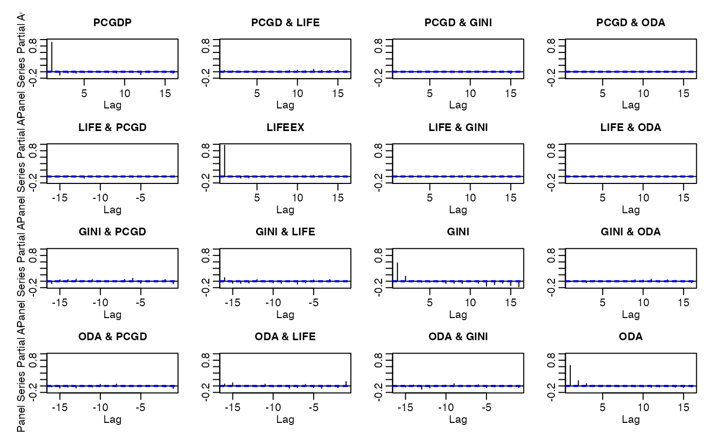
 pspacf(wlddev, ~country, ~year, cols = 9:12) # Partial panel-autocorrelations
 psmat(wlddev, ~iso3c, ~year, cols = 9:12) |> plot() # Convert panel to 3D array and plot
 ## collapse offers a few very efficent functions for data manipulation:
# Fast selecting and replacing columns
series <- get_vars(wlddev, 9:12) # Same as wlddev[9:12] but 2x faster
series <- fselect(wlddev, PCGDP:ODA) # Same thing: > 100x faster than dplyr::select
get_vars(wlddev, 9:12) <- series # Replace, 8x faster wlddev[9:12] <- series + replaces names
fselect(wlddev, PCGDP:ODA) <- series # Same thing
# Fast subsetting
head(fsubset(wlddev, country == "Ireland", -country, -iso3c))
#> date year decade region income OECD PCGDP LIFEEX
#> 1 1961-01-01 1960 1960 Europe & Central Asia High income TRUE NA 69.79651
#> 2 1962-01-01 1961 1960 Europe & Central Asia High income TRUE NA 69.97827
#> 3 1963-01-01 1962 1960 Europe & Central Asia High income TRUE NA 70.13407
#> 4 1964-01-01 1963 1960 Europe & Central Asia High income TRUE NA 70.27293
#> 5 1965-01-01 1964 1960 Europe & Central Asia High income TRUE NA 70.40129
#> 6 1966-01-01 1965 1960 Europe & Central Asia High income TRUE NA 70.52315
#> GINI ODA POP
#> 1 NA NA 2828600
#> 2 NA NA 2824400
#> 3 NA NA 2836050
#> 4 NA NA 2852650
#> 5 NA NA 2866550
#> 6 NA NA 2877300
head(fsubset(wlddev, country == "Ireland" & year > 1990, year, PCGDP:ODA))
#> year PCGDP LIFEEX GINI ODA
#> 1 1991 24642.11 75.00527 NA NA
#> 2 1992 25292.81 75.18095 NA NA
#> 3 1993 25844.34 75.33612 NA NA
#> 4 1994 27224.37 75.47680 36.9 NA
#> 5 1995 29694.65 75.61756 37.0 NA
#> 6 1996 31644.89 75.83171 35.6 NA
ss(wlddev, 1:10, 1:10) # This is an order of magnitude faster than wlddev[1:10, 1:10]
#> country iso3c date year decade region income OECD PCGDP
#> 1 Afghanistan AFG 1961-01-01 1960 1960 South Asia Low income FALSE NA
#> 2 Afghanistan AFG 1962-01-01 1961 1960 South Asia Low income FALSE NA
#> 3 Afghanistan AFG 1963-01-01 1962 1960 South Asia Low income FALSE NA
#> 4 Afghanistan AFG 1964-01-01 1963 1960 South Asia Low income FALSE NA
#> 5 Afghanistan AFG 1965-01-01 1964 1960 South Asia Low income FALSE NA
#> 6 Afghanistan AFG 1966-01-01 1965 1960 South Asia Low income FALSE NA
#> 7 Afghanistan AFG 1967-01-01 1966 1960 South Asia Low income FALSE NA
#> LIFEEX
#> 1 32.446
#> 2 32.962
#> 3 33.471
#> 4 33.971
#> 5 34.463
#> 6 34.948
#> 7 35.430
#> [ reached 'max' / getOption("max.print") -- omitted 3 rows ]
# Fast transforming
head(ftransform(wlddev, ODA_GDP = ODA / PCGDP, ODA_LIFEEX = sqrt(ODA) / LIFEEX))
#> Warning: NaNs produced
#> country iso3c date year decade region income OECD PCGDP
#> 1 Afghanistan AFG 1961-01-01 1960 1960 South Asia Low income FALSE NA
#> 2 Afghanistan AFG 1962-01-01 1961 1960 South Asia Low income FALSE NA
#> 3 Afghanistan AFG 1963-01-01 1962 1960 South Asia Low income FALSE NA
#> 4 Afghanistan AFG 1964-01-01 1963 1960 South Asia Low income FALSE NA
#> LIFEEX GINI ODA POP ODA_GDP ODA_LIFEEX
#> 1 32.446 NA 116769997 8996973 NA 333.0462
#> 2 32.962 NA 232080002 9169410 NA 462.1738
#> 3 33.471 NA 112839996 9351441 NA 317.3678
#> 4 33.971 NA 237720001 9543205 NA 453.8627
#> [ reached 'max' / getOption("max.print") -- omitted 2 rows ]
settransform(wlddev, ODA_GDP = ODA / PCGDP, ODA_LIFEEX = sqrt(ODA) / LIFEEX) # by reference
#> Warning: NaNs produced
head(ftransform(wlddev, PCGDP = NULL, ODA = NULL, GINI_sum = fsum(GINI)))
#> country iso3c date year decade region income OECD LIFEEX
#> 1 Afghanistan AFG 1961-01-01 1960 1960 South Asia Low income FALSE 32.446
#> 2 Afghanistan AFG 1962-01-01 1961 1960 South Asia Low income FALSE 32.962
#> 3 Afghanistan AFG 1963-01-01 1962 1960 South Asia Low income FALSE 33.471
#> 4 Afghanistan AFG 1964-01-01 1963 1960 South Asia Low income FALSE 33.971
#> 5 Afghanistan AFG 1965-01-01 1964 1960 South Asia Low income FALSE 34.463
#> GINI POP ODA_GDP ODA_LIFEEX GINI_sum
#> 1 NA 8996973 NA 333.0462 67203.5
#> 2 NA 9169410 NA 462.1738 67203.5
#> 3 NA 9351441 NA 317.3678 67203.5
#> 4 NA 9543205 NA 453.8627 67203.5
#> 5 NA 9744781 NA 499.1535 67203.5
#> [ reached 'max' / getOption("max.print") -- omitted 1 rows ]
head(ftransformv(wlddev, 9:12, log)) # Can also transform with lists of columns
#> Warning: NaNs produced
#> country iso3c date year decade region income OECD PCGDP
#> 1 Afghanistan AFG 1961-01-01 1960 1960 South Asia Low income FALSE NA
#> 2 Afghanistan AFG 1962-01-01 1961 1960 South Asia Low income FALSE NA
#> 3 Afghanistan AFG 1963-01-01 1962 1960 South Asia Low income FALSE NA
#> 4 Afghanistan AFG 1964-01-01 1963 1960 South Asia Low income FALSE NA
#> LIFEEX GINI ODA POP ODA_GDP ODA_LIFEEX
#> 1 3.479577 NA 18.57572 8996973 NA 333.0462
#> 2 3.495355 NA 19.26259 9169410 NA 462.1738
#> 3 3.510679 NA 18.54148 9351441 NA 317.3678
#> 4 3.525507 NA 19.28660 9543205 NA 453.8627
#> [ reached 'max' / getOption("max.print") -- omitted 2 rows ]
head(ftransformv(wlddev, 9:12, fscale, apply = FALSE)) # apply = FALSE invokes fscale.data.frame
#> country iso3c date year decade region income OECD PCGDP
#> 1 Afghanistan AFG 1961-01-01 1960 1960 South Asia Low income FALSE NA
#> 2 Afghanistan AFG 1962-01-01 1961 1960 South Asia Low income FALSE NA
#> 3 Afghanistan AFG 1963-01-01 1962 1960 South Asia Low income FALSE NA
#> 4 Afghanistan AFG 1964-01-01 1963 1960 South Asia Low income FALSE NA
#> LIFEEX GINI ODA POP ODA_GDP ODA_LIFEEX
#> 1 -2.775283 NA -0.3890241 8996973 NA 333.0462
#> 2 -2.730321 NA -0.2562874 9169410 NA 462.1738
#> 3 -2.685969 NA -0.3935480 9351441 NA 317.3678
#> 4 -2.642402 NA -0.2497951 9543205 NA 453.8627
#> [ reached 'max' / getOption("max.print") -- omitted 2 rows ]
settransformv(wlddev, 9:12, fscale, apply = FALSE) # Changing the data by reference
ftransform(wlddev) <- fscale(gv(wlddev, 9:12)) # Same thing (using replacement method)
library(magrittr) # Same thing, using magrittr
wlddev %<>% ftransformv(9:12, fscale, apply = FALSE)
wlddev %>% ftransform(gv(., 9:12) |> # With compound pipes: Scaling and lagging
fscale() |> flag(0:2, iso3c, year)) |> head()
#> country iso3c date year decade region income OECD PCGDP
#> 1 Afghanistan AFG 1961-01-01 1960 1960 South Asia Low income FALSE NA
#> 2 Afghanistan AFG 1962-01-01 1961 1960 South Asia Low income FALSE NA
#> 3 Afghanistan AFG 1963-01-01 1962 1960 South Asia Low income FALSE NA
#> LIFEEX GINI ODA POP ODA_GDP ODA_LIFEEX L1.PCGDP L2.PCGDP
#> 1 -2.775283 NA -0.3890241 8996973 NA 333.0462 NA NA
#> 2 -2.730321 NA -0.2562874 9169410 NA 462.1738 NA NA
#> 3 -2.685969 NA -0.3935480 9351441 NA 317.3678 NA NA
#> L1.LIFEEX L2.LIFEEX L1.GINI L2.GINI L1.ODA L2.ODA
#> 1 NA NA NA NA NA NA
#> 2 -2.775283 NA NA NA -0.3890241 NA
#> 3 -2.730321 -2.775283 NA NA -0.2562874 -0.3890241
#> [ reached 'max' / getOption("max.print") -- omitted 3 rows ]
# Fast reordering
head(roworder(wlddev, -country, year))
#> country iso3c date year decade region income
#> 1 Zimbabwe ZWE 1961-01-01 1960 1960 Sub-Saharan Africa Lower middle income
#> 2 Zimbabwe ZWE 1962-01-01 1961 1960 Sub-Saharan Africa Lower middle income
#> 3 Zimbabwe ZWE 1963-01-01 1962 1960 Sub-Saharan Africa Lower middle income
#> 4 Zimbabwe ZWE 1964-01-01 1963 1960 Sub-Saharan Africa Lower middle income
#> OECD PCGDP LIFEEX GINI ODA POP ODA_GDP ODA_LIFEEX
#> 1 FALSE -0.5794259 -0.9826503 NA NA 3776681 NA NA
#> 2 FALSE -0.5779547 -0.9422195 NA -0.5233262 3905034 97.77415 5.912678
#> 3 FALSE -0.5789920 -0.9018759 NA NA 4039201 NA NA
#> 4 FALSE -0.5775741 -0.8620551 NA -0.4094221 4178726 96162.61027 182.938198
#> [ reached 'max' / getOption("max.print") -- omitted 2 rows ]
head(colorder(wlddev, country, year))
#> country year iso3c date decade region income OECD PCGDP
#> 1 Afghanistan 1960 AFG 1961-01-01 1960 South Asia Low income FALSE NA
#> 2 Afghanistan 1961 AFG 1962-01-01 1960 South Asia Low income FALSE NA
#> 3 Afghanistan 1962 AFG 1963-01-01 1960 South Asia Low income FALSE NA
#> 4 Afghanistan 1963 AFG 1964-01-01 1960 South Asia Low income FALSE NA
#> LIFEEX GINI ODA POP ODA_GDP ODA_LIFEEX
#> 1 -2.775283 NA -0.3890241 8996973 NA 333.0462
#> 2 -2.730321 NA -0.2562874 9169410 NA 462.1738
#> 3 -2.685969 NA -0.3935480 9351441 NA 317.3678
#> 4 -2.642402 NA -0.2497951 9543205 NA 453.8627
#> [ reached 'max' / getOption("max.print") -- omitted 2 rows ]
# Fast renaming
head(frename(wlddev, country = Ctry, year = Yr))
#> Ctry iso3c date Yr decade region income OECD PCGDP
#> 1 Afghanistan AFG 1961-01-01 1960 1960 South Asia Low income FALSE NA
#> 2 Afghanistan AFG 1962-01-01 1961 1960 South Asia Low income FALSE NA
#> 3 Afghanistan AFG 1963-01-01 1962 1960 South Asia Low income FALSE NA
#> 4 Afghanistan AFG 1964-01-01 1963 1960 South Asia Low income FALSE NA
#> LIFEEX GINI ODA POP ODA_GDP ODA_LIFEEX
#> 1 -2.775283 NA -0.3890241 8996973 NA 333.0462
#> 2 -2.730321 NA -0.2562874 9169410 NA 462.1738
#> 3 -2.685969 NA -0.3935480 9351441 NA 317.3678
#> 4 -2.642402 NA -0.2497951 9543205 NA 453.8627
#> [ reached 'max' / getOption("max.print") -- omitted 2 rows ]
setrename(wlddev, country = Ctry, year = Yr) # By reference
head(frename(wlddev, tolower, cols = 9:12))
#> Ctry iso3c date Yr decade region income OECD pcgdp
#> 1 Afghanistan AFG 1961-01-01 1960 1960 South Asia Low income FALSE NA
#> 2 Afghanistan AFG 1962-01-01 1961 1960 South Asia Low income FALSE NA
#> 3 Afghanistan AFG 1963-01-01 1962 1960 South Asia Low income FALSE NA
#> 4 Afghanistan AFG 1964-01-01 1963 1960 South Asia Low income FALSE NA
#> lifeex gini oda POP ODA_GDP ODA_LIFEEX
#> 1 -2.775283 NA -0.3890241 8996973 NA 333.0462
#> 2 -2.730321 NA -0.2562874 9169410 NA 462.1738
#> 3 -2.685969 NA -0.3935480 9351441 NA 317.3678
#> 4 -2.642402 NA -0.2497951 9543205 NA 453.8627
#> [ reached 'max' / getOption("max.print") -- omitted 2 rows ]
# Fast grouping
fgroup_by(wlddev, Ctry, decade) |> fgroup_vars() |> head()
#> Ctry decade
#> 1 Afghanistan 1960
#> 2 Afghanistan 1960
#> 3 Afghanistan 1960
#> 4 Afghanistan 1960
#> 5 Afghanistan 1960
#> 6 Afghanistan 1960
rm(wlddev) # .. but only works with collapse functions
## Now lets start putting things together
wlddev |> fsubset(year > 1990, region, income, PCGDP:ODA) |>
fgroup_by(region, income) |> fmean() # Fast aggregation using the mean
#> region income PCGDP LIFEEX GINI
#> 1 East Asia & Pacific High income 32671.0522 78.21996 32.95000
#> 2 East Asia & Pacific Lower middle income 1738.5111 65.45647 36.51972
#> 3 East Asia & Pacific Upper middle income 4575.8695 70.87431 40.64815
#> 4 Europe & Central Asia High income 40814.1215 77.67583 30.94218
#> 5 Europe & Central Asia Low income 695.7951 65.04128 32.13333
#> 6 Europe & Central Asia Lower middle income 1779.7149 68.79873 30.66176
#> 7 Europe & Central Asia Upper middle income 5182.1800 71.30199 34.85362
#> 8 Latin America & Caribbean High income 19864.5057 75.55674 48.35714
#> 9 Latin America & Caribbean Low income 1189.8492 58.97359 41.10000
#> 10 Latin America & Caribbean Lower middle income 1987.5292 69.31612 50.58125
#> 11 Latin America & Caribbean Upper middle income 6224.6674 72.58127 49.88547
#> ODA
#> 1 112194118
#> 2 509965862
#> 3 219146704
#> 4 321907195
#> 5 244539286
#> 6 395371417
#> 7 463652924
#> 8 31307379
#> 9 753747928
#> 10 559540257
#> 11 188305879
#> [ reached 'max' / getOption("max.print") -- omitted 12 rows ]
# Same thing using dplyr manipulation verbs
library(dplyr)
wlddev |> filter(year > 1990) |> select(region, income, PCGDP:ODA) |>
group_by(region,income) |> fmean() # This is already a lot faster than summarize_all(mean)
#> # A tibble: 23 × 6
#> region income PCGDP LIFEEX GINI ODA
#> <fct> <fct> <dbl> <dbl> <dbl> <dbl>
#> 1 East Asia & Pacific High income 32671. 78.2 33.0 112194118.
#> 2 East Asia & Pacific Lower middle income 1739. 65.5 36.5 509965862.
#> 3 East Asia & Pacific Upper middle income 4576. 70.9 40.6 219146704.
#> 4 Europe & Central Asia High income 40814. 77.7 30.9 321907195.
#> 5 Europe & Central Asia Low income 696. 65.0 32.1 244539286.
#> 6 Europe & Central Asia Lower middle income 1780. 68.8 30.7 395371417.
#> 7 Europe & Central Asia Upper middle income 5182. 71.3 34.9 463652924.
#> 8 Latin America & Caribbean High income 19865. 75.6 48.4 31307379.
#> 9 Latin America & Caribbean Low income 1190. 59.0 41.1 753747928.
#> 10 Latin America & Caribbean Lower middle income 1988. 69.3 50.6 559540257.
#> # ℹ 13 more rows
wlddev |> fsubset(year > 1990, region, income, PCGDP:POP) |>
fgroup_by(region, income) |> fmean(POP) # Weighted group means
#> region income sum.POP PCGDP
#> 1 East Asia & Pacific High income 6165902760 37889.3406
#> 2 East Asia & Pacific Lower middle income 13784998066 2135.6182
#> 3 East Asia & Pacific Upper middle income 40150644873 3769.4215
#> 4 Europe & Central Asia High income 13923291507 34583.4203
#> 5 Europe & Central Asia Low income 203224216 722.7351
#> 6 Europe & Central Asia Lower middle income 2399154808 2145.1352
#> 7 Europe & Central Asia Upper middle income 8919358306 8238.8391
#> 8 Latin America & Caribbean High income 842939686 13068.1667
#> 9 Latin America & Caribbean Low income 267125746 1193.5889
#> 10 Latin America & Caribbean Lower middle income 815192217 2011.6260
#> LIFEEX GINI ODA
#> 1 80.79250 32.81601 -79785907
#> 2 68.24548 36.40362 1060544119
#> 3 73.07773 40.38496 1229983586
#> 4 78.82923 32.27710 1107199019
#> 5 65.76604 32.22326 261043896
#> 6 68.98050 28.97857 556232624
#> 7 69.78322 38.66475 1187976647
#> 8 76.76809 48.85497 97880105
#> 9 59.34831 41.10000 794781510
#> 10 69.33538 50.52363 571015463
#> [ reached 'max' / getOption("max.print") -- omitted 13 rows ]
wlddev |> fsubset(year > 1990, region, income, PCGDP:POP) |>
fgroup_by(region, income) |> fsd(POP) # Weighted group standard deviations
#> region income sum.POP PCGDP
#> 1 East Asia & Pacific High income 6165902760 11619.90339
#> 2 East Asia & Pacific Lower middle income 13784998066 1074.84975
#> 3 East Asia & Pacific Upper middle income 40150644873 2374.39410
#> 4 Europe & Central Asia High income 13923291507 13593.46879
#> 5 Europe & Central Asia Low income 203224216 238.47730
#> 6 Europe & Central Asia Lower middle income 2399154808 841.97662
#> 7 Europe & Central Asia Upper middle income 8919358306 3175.38606
#> 8 Latin America & Caribbean High income 842939686 6273.64310
#> 9 Latin America & Caribbean Low income 267125746 70.56928
#> 10 Latin America & Caribbean Lower middle income 815192217 580.31064
#> LIFEEX GINI ODA
#> 1 2.730868 1.247116 129087430
#> 2 4.230245 4.316708 943798728
#> 3 2.428883 2.458222 1519636778
#> 4 2.895801 2.994940 1131585991
#> 5 4.555972 1.547793 112926454
#> 6 1.688117 4.573107 370416116
#> 7 3.707457 4.227846 1068502287
#> 8 2.421882 5.289102 71662290
#> 9 2.815436 0.000000 566758933
#> 10 4.220554 5.684628 243414533
#> [ reached 'max' / getOption("max.print") -- omitted 13 rows ]
wlddev |> na_omit(cols = "POP") |> fgroup_by(region, income) |>
fselect(PCGDP:POP) |> fnth(0.75, POP) # Weighted group third quartile
#> region income sum.POP PCGDP LIFEEX
#> 1 East Asia & Pacific High income 11407808149 42201.079 81.71320
#> 2 East Asia & Pacific Lower middle income 22174820629 2350.332 69.84968
#> 3 East Asia & Pacific Upper middle income 69639871478 3796.016 73.77902
#> 4 Europe & Central Asia High income 27285316560 37939.285 79.12994
#> 5 Europe & Central Asia Low income 311485944 1010.399 68.74935
#> 6 Europe & Central Asia Lower middle income 4511786205 3049.405 70.15657
#> 7 Europe & Central Asia Upper middle income 16972478305 10543.823 70.57815
#> 8 Latin America & Caribbean High income 1466292826 13929.260 77.62527
#> 9 Latin America & Caribbean Low income 429756890 1426.615 60.19115
#> 10 Latin America & Caribbean Lower middle income 1290800630 2241.730 71.18339
#> GINI ODA
#> 1 33.50000 744862041
#> 2 39.09699 1828537218
#> 3 42.25373 2498289114
#> 4 34.70000 1665332268
#> 5 33.54169 369881699
#> 6 29.76143 713578745
#> 7 41.20000 1780829097
#> 8 54.82206 156066838
#> 9 41.10000 956301069
#> 10 55.50000 657517519
#> [ reached 'max' / getOption("max.print") -- omitted 13 rows ]
wlddev |> fgroup_by(country) |> fselect(PCGDP:ODA) |>
fwithin() |> head() # Within transformation
#> PCGDP LIFEEX GINI ODA
#> 1 NA -16.75117 NA -1370778502
#> 2 NA -16.23517 NA -1255468497
#> 3 NA -15.72617 NA -1374708502
#> 4 NA -15.22617 NA -1249828497
#> 5 NA -14.73417 NA -1191628485
#> 6 NA -14.24917 NA -1145708502
wlddev |> fgroup_by(country) |> fselect(PCGDP:ODA) |>
fmedian(TRA = "-") |> head() # Grouped centering using the median
#> PCGDP LIFEEX GINI ODA
#> 1 NA -17.5395 NA -144765007
#> 2 NA -17.0235 NA -29455002
#> 3 NA -16.5145 NA -148695007
#> 4 NA -16.0145 NA -23815002
#> 5 NA -15.5225 NA 34385010
#> 6 NA -15.0375 NA 80304993
# Replacing data points by the weighted first quartile:
wlddev |> na_omit(cols = "POP") |> fgroup_by(country) |>
fselect(country, year, PCGDP:POP) %>%
ftransform(fselect(., -country, -year) |>
fnth(0.25, POP, "fill")) |> head()
#> country year PCGDP LIFEEX GINI ODA POP
#> 1 Afghanistan 1960 406.9948 45.86685 NA 237899441 8996973
#> 2 Afghanistan 1961 406.9948 45.86685 NA 237899441 9169410
#> 3 Afghanistan 1962 406.9948 45.86685 NA 237899441 9351441
#> 4 Afghanistan 1963 406.9948 45.86685 NA 237899441 9543205
#> 5 Afghanistan 1964 406.9948 45.86685 NA 237899441 9744781
#> 6 Afghanistan 1965 406.9948 45.86685 NA 237899441 9956320
wlddev |> fgroup_by(country) |> fselect(PCGDP:ODA) |> fscale() |> head() # Standardizing
#> PCGDP LIFEEX GINI ODA
#> 1 NA -1.653181 NA -0.6498451
#> 2 NA -1.602256 NA -0.5951801
#> 3 NA -1.552023 NA -0.6517082
#> 4 NA -1.502678 NA -0.5925063
#> 5 NA -1.454122 NA -0.5649154
#> 6 NA -1.406257 NA -0.5431461
wlddev |> fgroup_by(country) |> fselect(PCGDP:POP) |>
fscale(POP) |> head() # Weighted..
#> POP PCGDP LIFEEX GINI ODA
#> 1 8996973 NA -2.172769 NA -0.9502811
#> 2 9169410 NA -2.119489 NA -0.9011481
#> 3 9351441 NA -2.066932 NA -0.9519557
#> 4 9543205 NA -2.015304 NA -0.8987449
#> 5 9744781 NA -1.964502 NA -0.8739462
#> 6 9956320 NA -1.914423 NA -0.8543799
wlddev |> fselect(country, year, PCGDP:ODA) |> # Adding 1 lead and 2 lags of each variable
fgroup_by(country) |> flag(-1:2, year) |> head()
#> country year F1.PCGDP PCGDP L1.PCGDP L2.PCGDP F1.LIFEEX LIFEEX L1.LIFEEX
#> 1 Afghanistan 1960 NA NA NA NA 32.962 32.446 NA
#> 2 Afghanistan 1961 NA NA NA NA 33.471 32.962 32.446
#> 3 Afghanistan 1962 NA NA NA NA 33.971 33.471 32.962
#> L2.LIFEEX F1.GINI GINI L1.GINI L2.GINI F1.ODA ODA L1.ODA
#> 1 NA NA NA NA NA 232080002 116769997 NA
#> 2 NA NA NA NA NA 112839996 232080002 116769997
#> 3 32.446 NA NA NA NA 237720001 112839996 232080002
#> L2.ODA
#> 1 NA
#> 2 NA
#> 3 116769997
#> [ reached 'max' / getOption("max.print") -- omitted 3 rows ]
wlddev |> fselect(country, year, PCGDP:ODA) |> # Adding 1 lead and 10-year growth rates
fgroup_by(country) |> fgrowth(c(0:1,10), 1, year) |> head()
#> country year PCGDP G1.PCGDP L10G1.PCGDP LIFEEX G1.LIFEEX L10G1.LIFEEX
#> 1 Afghanistan 1960 NA NA NA 32.446 NA NA
#> 2 Afghanistan 1961 NA NA NA 32.962 1.590335 NA
#> 3 Afghanistan 1962 NA NA NA 33.471 1.544202 NA
#> 4 Afghanistan 1963 NA NA NA 33.971 1.493830 NA
#> 5 Afghanistan 1964 NA NA NA 34.463 1.448294 NA
#> GINI G1.GINI L10G1.GINI ODA G1.ODA L10G1.ODA
#> 1 NA NA NA 116769997 NA NA
#> 2 NA NA NA 232080002 98.74969 NA
#> 3 NA NA NA 112839996 -51.37884 NA
#> 4 NA NA NA 237720001 110.66998 NA
#> 5 NA NA NA 295920013 24.48259 NA
#> [ reached 'max' / getOption("max.print") -- omitted 1 rows ]
# etc...
# Aggregation with multiple functions
wlddev |> fsubset(year > 1990, region, income, PCGDP:ODA) |>
fgroup_by(region, income) %>% {
add_vars(fgroup_vars(., "unique"),
fmedian(., keep.group_vars = FALSE) |> add_stub("median_"),
fmean(., keep.group_vars = FALSE) |> add_stub("mean_"),
fsd(., keep.group_vars = FALSE) |> add_stub("sd_"))
} |> head()
#> region income median_PCGDP median_LIFEEX
#> 1 East Asia & Pacific High income 32573.8177 78.54024
#> 2 East Asia & Pacific Lower middle income 1658.3786 66.07200
#> 3 East Asia & Pacific Upper middle income 3583.2189 70.61500
#> 4 Europe & Central Asia High income 36201.7707 78.16061
#> 5 Europe & Central Asia Low income 668.9513 66.08000
#> median_GINI median_ODA mean_PCGDP mean_LIFEEX mean_GINI mean_ODA sd_PCGDP
#> 1 32.75 11500000 32671.0522 78.21996 32.95000 112194118 13031.1867
#> 2 35.70 257079987 1738.5111 65.45647 36.51972 509965862 904.3004
#> 3 40.35 49730000 4575.8695 70.87431 40.64815 219146704 2489.3795
#> 4 31.10 138889999 40814.1215 77.67583 30.94218 321907195 29485.3091
#> 5 32.45 239055000 695.7951 65.04128 32.13333 244539286 242.4158
#> sd_LIFEEX sd_GINI sd_ODA
#> 1 3.825737 1.322624 223580786
#> 2 5.003373 4.779528 686619373
#> 3 3.157915 3.506637 684346804
#> 4 3.810700 3.676878 632730086
#> 5 4.723263 1.713087 116363515
#> [ reached 'max' / getOption("max.print") -- omitted 1 rows ]
# Transformation with multiple functions
wlddev |> fselect(country, year, PCGDP:ODA) |>
fgroup_by(country) %>% {
add_vars(fdiff(., c(1,10), 1, year) |> flag(0:2, year), # Sequence of lagged differences
ftransform(., fselect(., PCGDP:ODA) |> fwithin() |> add_stub("W.")) |>
flag(0:2, year, keep.ids = FALSE)) # Sequence of lagged demeaned vars
} |> head()
#> country year D1.PCGDP L1.D1.PCGDP L2.D1.PCGDP L10D1.PCGDP L1.L10D1.PCGDP
#> 1 Afghanistan 1960 NA NA NA NA NA
#> L2.L10D1.PCGDP D1.LIFEEX L1.D1.LIFEEX L2.D1.LIFEEX L10D1.LIFEEX
#> 1 NA NA NA NA NA
#> L1.L10D1.LIFEEX L2.L10D1.LIFEEX D1.GINI L1.D1.GINI L2.D1.GINI L10D1.GINI
#> 1 NA NA NA NA NA NA
#> L1.L10D1.GINI L2.L10D1.GINI D1.ODA L1.D1.ODA L2.D1.ODA L10D1.ODA L1.L10D1.ODA
#> 1 NA NA NA NA NA NA NA
#> L2.L10D1.ODA PCGDP L1.PCGDP L2.PCGDP LIFEEX L1.LIFEEX L2.LIFEEX GINI L1.GINI
#> 1 NA NA NA NA 32.446 NA NA NA NA
#> L2.GINI ODA L1.ODA L2.ODA W.PCGDP L1.W.PCGDP L2.W.PCGDP W.LIFEEX
#> 1 NA 116769997 NA NA NA NA NA -16.75117
#> L1.W.LIFEEX L2.W.LIFEEX W.GINI L1.W.GINI L2.W.GINI W.ODA L1.W.ODA
#> 1 NA NA NA NA NA -1370778502 NA
#> L2.W.ODA
#> 1 NA
#> [ reached 'max' / getOption("max.print") -- omitted 5 rows ]
# With ftransform, can also easily do one or more grouped mutations on the fly..
settransform(wlddev, median_ODA = fmedian(ODA, list(region, income), TRA = "fill"))
settransform(wlddev, sd_ODA = fsd(ODA, list(region, income), TRA = "fill"),
mean_GDP = fmean(PCGDP, country, TRA = "fill"))
wlddev %<>% ftransform(fmedian(list(median_ODA = ODA, median_GDP = PCGDP),
list(region, income), TRA = "fill"))
# On a groped data frame it is also possible to grouped transform certain columns
# but perform aggregate operatins on others:
wlddev |> fgroup_by(region, income) %>%
ftransform(gmedian_GDP = fmedian(PCGDP, GRP(.), TRA = "replace"),
omedian_GDP = fmedian(PCGDP, TRA = "replace"), # "replace" preserves NA's
omedian_GDP_fill = fmedian(PCGDP)) |> tail()
#> country iso3c date year decade region
#> 13171 Zimbabwe ZWE 2016-01-01 2015 2010 Sub-Saharan Africa
#> 13172 Zimbabwe ZWE 2017-01-01 2016 2010 Sub-Saharan Africa
#> 13173 Zimbabwe ZWE 2018-01-01 2017 2010 Sub-Saharan Africa
#> income OECD PCGDP LIFEEX GINI ODA POP
#> 13171 Lower middle income FALSE 1234.103 59.534 NA 817729980 13814629
#> 13172 Lower middle income FALSE 1224.310 60.294 NA 687659973 14030390
#> 13173 Lower middle income FALSE 1263.321 60.812 44.3 753909973 14236745
#> median_ODA sd_ODA mean_GDP median_GDP gmedian_GDP omedian_GDP
#> 13171 280630005 694376321 1219.436 1336.053 1336.053 3767.162
#> 13172 280630005 694376321 1219.436 1336.053 1336.053 3767.162
#> 13173 280630005 694376321 1219.436 1336.053 1336.053 3767.162
#> omedian_GDP_fill
#> 13171 3767.162
#> 13172 3767.162
#> 13173 3767.162
#> [ reached 'max' / getOption("max.print") -- omitted 3 rows ]
rm(wlddev)
## For multi-type data aggregation, the function collap() offers ease and flexibility
# Aggregate this data by country and decade: Numeric columns with mean, categorical with mode
head(collap(wlddev, ~ country + decade, fmean, fmode))
#> country iso3c date year decade region income OECD
#> 1 Afghanistan AFG 1961-01-01 1964.5 1960 South Asia Low income FALSE
#> 2 Afghanistan AFG 1971-01-01 1974.5 1970 South Asia Low income FALSE
#> 3 Afghanistan AFG 1981-01-01 1984.5 1980 South Asia Low income FALSE
#> 4 Afghanistan AFG 1991-01-01 1994.5 1990 South Asia Low income FALSE
#> 5 Afghanistan AFG 2001-01-01 2004.5 2000 South Asia Low income FALSE
#> PCGDP LIFEEX GINI ODA POP
#> 1 NA 34.6908 NA 222288999 9886773
#> 2 NA 39.9053 NA 236169998 12451803
#> 3 NA 46.4176 NA 71666001 12291854
#> 4 NA 53.0097 NA 317255000 16931903
#> 5 379.373 58.0881 NA 3054051961 24870022
#> [ reached 'max' / getOption("max.print") -- omitted 1 rows ]
# taking weighted mean and weighted mode:
head(collap(wlddev, ~ country + decade, fmean, fmode, w = ~ POP, wFUN = fsum))
#> country iso3c date year decade region income OECD
#> 1 Afghanistan AFG 1970-01-01 1964.675 1960 South Asia Low income FALSE
#> 2 Afghanistan AFG 1980-01-01 1974.672 1970 South Asia Low income FALSE
#> 3 Afghanistan AFG 1981-01-01 1984.364 1980 South Asia Low income FALSE
#> 4 Afghanistan AFG 2000-01-01 1994.941 1990 South Asia Low income FALSE
#> 5 Afghanistan AFG 2010-01-01 2004.788 2000 South Asia Low income FALSE
#> PCGDP LIFEEX GINI ODA POP
#> 1 NA 34.77716 NA 223006447 98867731
#> 2 NA 40.00367 NA 236798314 124518028
#> 3 NA 46.32098 NA 70613923 122918537
#> 4 NA 53.25897 NA 306818649 169319030
#> 5 382.5583 58.23630 NA 3240143310 248700217
#> [ reached 'max' / getOption("max.print") -- omitted 1 rows ]
# Multi-function aggregation of certain columns
head(collap(wlddev, ~ country + decade,
list(fmean, fmedian, fsd),
list(ffirst, flast), cols = c(3,9:12)))
#> country ffirst.date flast.date decade fmean.PCGDP fmedian.PCGDP fsd.PCGDP
#> 1 Afghanistan 1961-01-01 1970-01-01 1960 NA NA NA
#> 2 Afghanistan 1971-01-01 1980-01-01 1970 NA NA NA
#> 3 Afghanistan 1981-01-01 1990-01-01 1980 NA NA NA
#> 4 Afghanistan 1991-01-01 2000-01-01 1990 NA NA NA
#> fmean.LIFEEX fmedian.LIFEEX fsd.LIFEEX fmean.GINI fmedian.GINI fsd.GINI
#> 1 34.6908 34.7055 1.490964 NA NA NA
#> 2 39.9053 39.8430 1.738383 NA NA NA
#> 3 46.4176 46.4005 2.161460 NA NA NA
#> 4 53.0097 53.1200 1.695424 NA NA NA
#> fmean.ODA fmedian.ODA fsd.ODA
#> 1 222288999 234900002 80884369
#> 2 236169998 246509995 34241008
#> 3 71666001 48539999 72958531
#> 4 317255000 285175003 160500141
#> [ reached 'max' / getOption("max.print") -- omitted 2 rows ]
# Customized Aggregation: Assign columns to functions
head(collap(wlddev, ~ country + decade,
custom = list(fmean = 9:10, fsd = 9:12, flast = 3, ffirst = 6:8)))
#> country flast.date decade ffirst.region ffirst.income ffirst.OECD
#> 1 Afghanistan 1970-01-01 1960 South Asia Low income FALSE
#> 2 Afghanistan 1980-01-01 1970 South Asia Low income FALSE
#> 3 Afghanistan 1990-01-01 1980 South Asia Low income FALSE
#> 4 Afghanistan 2000-01-01 1990 South Asia Low income FALSE
#> 5 Afghanistan 2010-01-01 2000 South Asia Low income FALSE
#> fmean.PCGDP fsd.PCGDP fmean.LIFEEX fsd.LIFEEX fsd.GINI fsd.ODA
#> 1 NA NA 34.6908 1.490964 NA 80884369
#> 2 NA NA 39.9053 1.738383 NA 34241008
#> 3 NA NA 46.4176 2.161460 NA 72958531
#> 4 NA NA 53.0097 1.695424 NA 160500141
#> 5 379.373 53.66524 58.0881 1.565630 NA 2013110021
#> [ reached 'max' / getOption("max.print") -- omitted 1 rows ]
# For grouped data frames use collapg
wlddev |> fsubset(year > 1990, country, region, income, PCGDP:ODA) |>
fgroup_by(country) |> collapg(fmean, ffirst) |>
ftransform(AMGDP = PCGDP > fmedian(PCGDP, list(region, income), TRA = "fill"),
AMODA = ODA > fmedian(ODA, income, TRA = "replace_fill")) |> head()
#> country region income PCGDP
#> 1 Afghanistan South Asia Low income 483.8351
#> 2 Albania Europe & Central Asia Upper middle income 3127.1510
#> 3 Algeria Middle East & North Africa Upper middle income 4056.4341
#> 4 American Samoa East Asia & Pacific Upper middle income 10071.0659
#> 5 Andorra Europe & Central Asia High income 40768.8453
#> 6 Angola Sub-Saharan Africa Lower middle income 2876.5065
#> LIFEEX GINI ODA AMGDP AMODA
#> 1 58.32283 NA 2888193791 FALSE TRUE
#> 2 75.19266 31.41111 343797587 FALSE TRUE
#> 3 72.57717 31.45000 287459654 FALSE TRUE
#> 4 NA NA NA TRUE NA
#> 5 NA NA NA TRUE NA
#> 6 51.59572 48.66667 412104483 TRUE FALSE
## Additional flexibility for data transformation tasks is offerend by tidy transformation operators
# Within-transformation (centering on overall mean)
head(W(wlddev, ~ country, cols = 9:12, mean = "overall.mean"))
#> country W.PCGDP W.LIFEEX W.GINI W.ODA
#> 1 Afghanistan NA 47.54514 NA -916058371
#> 2 Afghanistan NA 48.06114 NA -800748366
#> 3 Afghanistan NA 48.57014 NA -919988371
#> 4 Afghanistan NA 49.07014 NA -795108366
#> 5 Afghanistan NA 49.56214 NA -736908354
#> 6 Afghanistan NA 50.04714 NA -690988371
# Partialling out country and year fixed effects
head(HDW(wlddev, PCGDP + LIFEEX ~ qF(country) + qF(year)))
#> HDW.PCGDP HDW.LIFEEX
#> 1 1578.6211 -1.3980224
#> 2 1412.8849 -1.1838196
#> 3 917.2033 -1.0547978
#> 4 627.8605 -0.8296048
#> 5 168.0458 -0.6683027
#> 6 -234.9535 -0.4708428
# Same, adding ODA as continuous regressor
head(HDW(wlddev, PCGDP + LIFEEX ~ qF(country) + qF(year) + ODA))
#> HDW.PCGDP HDW.LIFEEX
#> 1 -324.3991 -1.1765307
#> 2 -439.5404 -0.9751559
#> 3 -598.9266 -0.7835446
#> 4 100.2175 -0.6186010
#> 5 -70.7664 -0.4966332
#> 6 330.3561 -0.2257800
# Standardizing (scaling and centering) by country
head(STD(wlddev, ~ country, cols = 9:12))
#> country STD.PCGDP STD.LIFEEX STD.GINI STD.ODA
#> 1 Afghanistan NA -1.653181 NA -0.6498451
#> 2 Afghanistan NA -1.602256 NA -0.5951801
#> 3 Afghanistan NA -1.552023 NA -0.6517082
#> 4 Afghanistan NA -1.502678 NA -0.5925063
#> 5 Afghanistan NA -1.454122 NA -0.5649154
#> 6 Afghanistan NA -1.406257 NA -0.5431461
# Computing 1 lead and 3 lags of the 4 series
head(L(wlddev, -1:3, ~ country, ~year, cols = 9:12))
#> country year F1.PCGDP PCGDP L1.PCGDP L2.PCGDP L3.PCGDP F1.LIFEEX LIFEEX
#> 1 Afghanistan 1960 NA NA NA NA NA 32.962 32.446
#> 2 Afghanistan 1961 NA NA NA NA NA 33.471 32.962
#> 3 Afghanistan 1962 NA NA NA NA NA 33.971 33.471
#> L1.LIFEEX L2.LIFEEX L3.LIFEEX F1.GINI GINI L1.GINI L2.GINI L3.GINI F1.ODA
#> 1 NA NA NA NA NA NA NA NA 232080002
#> 2 32.446 NA NA NA NA NA NA NA 112839996
#> 3 32.962 32.446 NA NA NA NA NA NA 237720001
#> ODA L1.ODA L2.ODA L3.ODA
#> 1 116769997 NA NA NA
#> 2 232080002 116769997 NA NA
#> 3 112839996 232080002 116769997 NA
#> [ reached 'max' / getOption("max.print") -- omitted 3 rows ]
# Computing the 1- and 10-year first differences
head(D(wlddev, c(1,10), 1, ~ country, ~year, cols = 9:12))
#> country year D1.PCGDP L10D1.PCGDP D1.LIFEEX L10D1.LIFEEX D1.GINI
#> 1 Afghanistan 1960 NA NA NA NA NA
#> 2 Afghanistan 1961 NA NA 0.516 NA NA
#> 3 Afghanistan 1962 NA NA 0.509 NA NA
#> 4 Afghanistan 1963 NA NA 0.500 NA NA
#> 5 Afghanistan 1964 NA NA 0.492 NA NA
#> 6 Afghanistan 1965 NA NA 0.485 NA NA
#> L10D1.GINI D1.ODA L10D1.ODA
#> 1 NA NA NA
#> 2 NA 115310005 NA
#> 3 NA -119240005 NA
#> 4 NA 124880005 NA
#> 5 NA 58200012 NA
#> 6 NA 45919983 NA
head(D(wlddev, c(1,10), 1:2, ~ country, ~year, cols = 9:12)) # ..first and second differences
#> country year D1.PCGDP D2.PCGDP L10D1.PCGDP L10D2.PCGDP D1.LIFEEX
#> 1 Afghanistan 1960 NA NA NA NA NA
#> 2 Afghanistan 1961 NA NA NA NA 0.516
#> 3 Afghanistan 1962 NA NA NA NA 0.509
#> D2.LIFEEX L10D1.LIFEEX L10D2.LIFEEX D1.GINI D2.GINI L10D1.GINI L10D2.GINI
#> 1 NA NA NA NA NA NA NA
#> 2 NA NA NA NA NA NA NA
#> 3 -0.007 NA NA NA NA NA NA
#> D1.ODA D2.ODA L10D1.ODA L10D2.ODA
#> 1 NA NA NA NA
#> 2 115310005 NA NA NA
#> 3 -119240005 -234550011 NA NA
#> [ reached 'max' / getOption("max.print") -- omitted 3 rows ]
# Computing the 1- and 10-year growth rates
head(G(wlddev, c(1,10), 1, ~ country, ~year, cols = 9:12))
#> country year G1.PCGDP L10G1.PCGDP G1.LIFEEX L10G1.LIFEEX G1.GINI
#> 1 Afghanistan 1960 NA NA NA NA NA
#> 2 Afghanistan 1961 NA NA 1.590335 NA NA
#> 3 Afghanistan 1962 NA NA 1.544202 NA NA
#> 4 Afghanistan 1963 NA NA 1.493830 NA NA
#> 5 Afghanistan 1964 NA NA 1.448294 NA NA
#> 6 Afghanistan 1965 NA NA 1.407306 NA NA
#> L10G1.GINI G1.ODA L10G1.ODA
#> 1 NA NA NA
#> 2 NA 98.74969 NA
#> 3 NA -51.37884 NA
#> 4 NA 110.66998 NA
#> 5 NA 24.48259 NA
#> 6 NA 15.51770 NA
# Adding growth rate variables to dataset
add_vars(wlddev) <- G(wlddev, c(1, 10), 1, ~ country, ~year, cols = 9:12, keep.ids = FALSE)
get_vars(wlddev, "G1.", regex = TRUE) <- NULL # Deleting again
# These operators can conveniently be used in regression formulas:
# Using a Mundlak (1978) procedure to estimate the effect of OECD on LIFEEX, controlling for PCGDP
lm(LIFEEX ~ log(PCGDP) + OECD + B(log(PCGDP), country),
wlddev |> fselect(country, OECD, PCGDP, LIFEEX) |> na_omit())
#>
#> Call:
#> lm(formula = LIFEEX ~ log(PCGDP) + OECD + B(log(PCGDP), country),
#> data = na_omit(fselect(wlddev, country, OECD, PCGDP, LIFEEX)))
#>
#> Coefficients:
#> (Intercept) log(PCGDP) OECDTRUE
#> 19.32590 8.20551 0.02478
#> B(log(PCGDP), country)
#> -2.65428
#>
# Adding 10-year lagged life-expectancy to allow for some convergence effects (dynamic panel model)
lm(LIFEEX ~ L(LIFEEX, 10, country) + log(PCGDP) + OECD + B(log(PCGDP), country),
wlddev |> fselect(country, OECD, PCGDP, LIFEEX) |> na_omit())
#>
#> Call:
#> lm(formula = LIFEEX ~ L(LIFEEX, 10, country) + log(PCGDP) + OECD +
#> B(log(PCGDP), country), data = na_omit(fselect(wlddev, country,
#> OECD, PCGDP, LIFEEX)))
#>
#> Coefficients:
#> (Intercept) L(LIFEEX, 10, country) log(PCGDP)
#> 9.2756 0.8656 0.9229
#> OECDTRUE B(log(PCGDP), country)
#> 0.4158 -0.6581
#>
# Tranformation functions and operators also support indexed data classes:
wldi <- findex_by(wlddev, country, year)
head(W(wldi$PCGDP)) # Country-demeaning
#> [1] NA NA NA NA NA NA
#>
#> Indexed by: country [1] | year [6 (61)]
head(W(wldi, cols = 9:12))
#> country year W.PCGDP W.LIFEEX W.GINI W.ODA
#> 1 Afghanistan 1960 NA -16.75117 NA -1370778502
#> 2 Afghanistan 1961 NA -16.23517 NA -1255468497
#> 3 Afghanistan 1962 NA -15.72617 NA -1374708502
#> 4 Afghanistan 1963 NA -15.22617 NA -1249828497
#> 5 Afghanistan 1964 NA -14.73417 NA -1191628485
#> 6 Afghanistan 1965 NA -14.24917 NA -1145708502
#>
#> Indexed by: country [1] | year [6 (61)]
head(W(wldi$PCGDP, effect = 2)) # Time-demeaning
#> [1] NA NA NA NA NA NA
#>
#> Indexed by: country [1] | year [6 (61)]
head(W(wldi, effect = 2, cols = 9:12))
#> country year W.PCGDP W.LIFEEX W.GINI W.ODA
#> 1 Afghanistan 1960 NA -21.46606 NA -122241092
#> 2 Afghanistan 1961 NA -21.51241 NA -37552049
#> 3 Afghanistan 1962 NA -21.38618 NA -183366702
#> 4 Afghanistan 1963 NA -21.23172 NA -54896550
#> 5 Afghanistan 1964 NA -21.20502 NA -9633789
#> 6 Afghanistan 1965 NA -21.18163 NA 5438669
#>
#> Indexed by: country [1] | year [6 (61)]
head(HDW(wldi$PCGDP)) # Country- and time-demeaning
#> [1] NA NA NA NA NA NA
#>
#> Indexed by: country [1] | year [6 (61)]
head(HDW(wldi, cols = 9:12))
#> HDW.PCGDP HDW.LIFEEX HDW.GINI HDW.ODA
#> 1 NA -6.706423 NA -1093922188
#> 2 NA -6.688440 NA -1032355993
#> 3 NA -6.562210 NA -1156945288
#> 4 NA -6.472079 NA -1046169271
#> 5 NA -6.445378 NA -996348510
#> 6 NA -6.367659 NA -983277444
#>
#> Indexed by: country [1] | year [6 (61)]
head(STD(wldi$PCGDP)) # Standardizing by country
#> [1] NA NA NA NA NA NA
#>
#> Indexed by: country [1] | year [6 (61)]
head(STD(wldi, cols = 9:12))
#> country year STD.PCGDP STD.LIFEEX STD.GINI STD.ODA
#> 1 Afghanistan 1960 NA -1.653181 NA -0.6498451
#> 2 Afghanistan 1961 NA -1.602256 NA -0.5951801
#> 3 Afghanistan 1962 NA -1.552023 NA -0.6517082
#> 4 Afghanistan 1963 NA -1.502678 NA -0.5925063
#> 5 Afghanistan 1964 NA -1.454122 NA -0.5649154
#> 6 Afghanistan 1965 NA -1.406257 NA -0.5431461
#>
#> Indexed by: country [1] | year [6 (61)]
head(L(wldi$PCGDP, -1:3)) # Panel-lags
#> F1 -- L1 L2 L3
#> [1,] NA NA NA NA NA
#> [2,] NA NA NA NA NA
#> [3,] NA NA NA NA NA
#> [4,] NA NA NA NA NA
#> [5,] NA NA NA NA NA
#> [6,] NA NA NA NA NA
#> attr(,"class")
#> [1] "matrix" "array"
#>
#> Indexed by: country [1] | year [6 (61)]
head(L(wldi, -1:3, 9:12))
#> country year F1.PCGDP PCGDP L1.PCGDP L2.PCGDP L3.PCGDP F1.LIFEEX LIFEEX
#> 1 Afghanistan 1960 NA NA NA NA NA 32.962 32.446
#> 2 Afghanistan 1961 NA NA NA NA NA 33.471 32.962
#> 3 Afghanistan 1962 NA NA NA NA NA 33.971 33.471
#> L1.LIFEEX L2.LIFEEX L3.LIFEEX F1.GINI GINI L1.GINI L2.GINI L3.GINI F1.ODA
#> 1 NA NA NA NA NA NA NA NA 232080002
#> 2 32.446 NA NA NA NA NA NA NA 112839996
#> 3 32.962 32.446 NA NA NA NA NA NA 237720001
#> ODA L1.ODA L2.ODA L3.ODA
#> 1 116769997 NA NA NA
#> 2 232080002 116769997 NA NA
#> 3 112839996 232080002 116769997 NA
#> [ reached 'max' / getOption("max.print") -- omitted 3 rows ]
#>
#> Indexed by: country [1] | year [6 (61)]
head(G(wldi$PCGDP)) # Panel-Growth rates
#> [1] NA NA NA NA NA NA
#>
#> Indexed by: country [1] | year [6 (61)]
head(G(wldi, 1, 1, 9:12))
#> country year G1.PCGDP G1.LIFEEX G1.GINI G1.ODA
#> 1 Afghanistan 1960 NA NA NA NA
#> 2 Afghanistan 1961 NA 1.590335 NA 98.74969
#> 3 Afghanistan 1962 NA 1.544202 NA -51.37884
#> 4 Afghanistan 1963 NA 1.493830 NA 110.66998
#> 5 Afghanistan 1964 NA 1.448294 NA 24.48259
#> 6 Afghanistan 1965 NA 1.407306 NA 15.51770
#>
#> Indexed by: country [1] | year [6 (61)]
lm(Dlog(PCGDP) ~ L(Dlog(LIFEEX), 0:3), wldi) # Panel data regression
#>
#> Call:
#> lm(formula = Dlog(PCGDP) ~ L(Dlog(LIFEEX), 0:3), data = wldi)
#>
#> Coefficients:
#> (Intercept) L(Dlog(LIFEEX), 0:3)-- L(Dlog(LIFEEX), 0:3)L1
#> 0.01544 -0.12618 0.38523
#> L(Dlog(LIFEEX), 0:3)L2 L(Dlog(LIFEEX), 0:3)L3
#> 0.54179 -0.16475
#>
rm(wldi)
# Remove all objects used in this example section
rm(v, d, w, f, f1, f2, g, mtcarsM, sds, series, wlddev)
## collapse offers a few very efficent functions for data manipulation:
# Fast selecting and replacing columns
series <- get_vars(wlddev, 9:12) # Same as wlddev[9:12] but 2x faster
series <- fselect(wlddev, PCGDP:ODA) # Same thing: > 100x faster than dplyr::select
get_vars(wlddev, 9:12) <- series # Replace, 8x faster wlddev[9:12] <- series + replaces names
fselect(wlddev, PCGDP:ODA) <- series # Same thing
# Fast subsetting
head(fsubset(wlddev, country == "Ireland", -country, -iso3c))
#> date year decade region income OECD PCGDP LIFEEX
#> 1 1961-01-01 1960 1960 Europe & Central Asia High income TRUE NA 69.79651
#> 2 1962-01-01 1961 1960 Europe & Central Asia High income TRUE NA 69.97827
#> 3 1963-01-01 1962 1960 Europe & Central Asia High income TRUE NA 70.13407
#> 4 1964-01-01 1963 1960 Europe & Central Asia High income TRUE NA 70.27293
#> 5 1965-01-01 1964 1960 Europe & Central Asia High income TRUE NA 70.40129
#> 6 1966-01-01 1965 1960 Europe & Central Asia High income TRUE NA 70.52315
#> GINI ODA POP
#> 1 NA NA 2828600
#> 2 NA NA 2824400
#> 3 NA NA 2836050
#> 4 NA NA 2852650
#> 5 NA NA 2866550
#> 6 NA NA 2877300
head(fsubset(wlddev, country == "Ireland" & year > 1990, year, PCGDP:ODA))
#> year PCGDP LIFEEX GINI ODA
#> 1 1991 24642.11 75.00527 NA NA
#> 2 1992 25292.81 75.18095 NA NA
#> 3 1993 25844.34 75.33612 NA NA
#> 4 1994 27224.37 75.47680 36.9 NA
#> 5 1995 29694.65 75.61756 37.0 NA
#> 6 1996 31644.89 75.83171 35.6 NA
ss(wlddev, 1:10, 1:10) # This is an order of magnitude faster than wlddev[1:10, 1:10]
#> country iso3c date year decade region income OECD PCGDP
#> 1 Afghanistan AFG 1961-01-01 1960 1960 South Asia Low income FALSE NA
#> 2 Afghanistan AFG 1962-01-01 1961 1960 South Asia Low income FALSE NA
#> 3 Afghanistan AFG 1963-01-01 1962 1960 South Asia Low income FALSE NA
#> 4 Afghanistan AFG 1964-01-01 1963 1960 South Asia Low income FALSE NA
#> 5 Afghanistan AFG 1965-01-01 1964 1960 South Asia Low income FALSE NA
#> 6 Afghanistan AFG 1966-01-01 1965 1960 South Asia Low income FALSE NA
#> 7 Afghanistan AFG 1967-01-01 1966 1960 South Asia Low income FALSE NA
#> LIFEEX
#> 1 32.446
#> 2 32.962
#> 3 33.471
#> 4 33.971
#> 5 34.463
#> 6 34.948
#> 7 35.430
#> [ reached 'max' / getOption("max.print") -- omitted 3 rows ]
# Fast transforming
head(ftransform(wlddev, ODA_GDP = ODA / PCGDP, ODA_LIFEEX = sqrt(ODA) / LIFEEX))
#> Warning: NaNs produced
#> country iso3c date year decade region income OECD PCGDP
#> 1 Afghanistan AFG 1961-01-01 1960 1960 South Asia Low income FALSE NA
#> 2 Afghanistan AFG 1962-01-01 1961 1960 South Asia Low income FALSE NA
#> 3 Afghanistan AFG 1963-01-01 1962 1960 South Asia Low income FALSE NA
#> 4 Afghanistan AFG 1964-01-01 1963 1960 South Asia Low income FALSE NA
#> LIFEEX GINI ODA POP ODA_GDP ODA_LIFEEX
#> 1 32.446 NA 116769997 8996973 NA 333.0462
#> 2 32.962 NA 232080002 9169410 NA 462.1738
#> 3 33.471 NA 112839996 9351441 NA 317.3678
#> 4 33.971 NA 237720001 9543205 NA 453.8627
#> [ reached 'max' / getOption("max.print") -- omitted 2 rows ]
settransform(wlddev, ODA_GDP = ODA / PCGDP, ODA_LIFEEX = sqrt(ODA) / LIFEEX) # by reference
#> Warning: NaNs produced
head(ftransform(wlddev, PCGDP = NULL, ODA = NULL, GINI_sum = fsum(GINI)))
#> country iso3c date year decade region income OECD LIFEEX
#> 1 Afghanistan AFG 1961-01-01 1960 1960 South Asia Low income FALSE 32.446
#> 2 Afghanistan AFG 1962-01-01 1961 1960 South Asia Low income FALSE 32.962
#> 3 Afghanistan AFG 1963-01-01 1962 1960 South Asia Low income FALSE 33.471
#> 4 Afghanistan AFG 1964-01-01 1963 1960 South Asia Low income FALSE 33.971
#> 5 Afghanistan AFG 1965-01-01 1964 1960 South Asia Low income FALSE 34.463
#> GINI POP ODA_GDP ODA_LIFEEX GINI_sum
#> 1 NA 8996973 NA 333.0462 67203.5
#> 2 NA 9169410 NA 462.1738 67203.5
#> 3 NA 9351441 NA 317.3678 67203.5
#> 4 NA 9543205 NA 453.8627 67203.5
#> 5 NA 9744781 NA 499.1535 67203.5
#> [ reached 'max' / getOption("max.print") -- omitted 1 rows ]
head(ftransformv(wlddev, 9:12, log)) # Can also transform with lists of columns
#> Warning: NaNs produced
#> country iso3c date year decade region income OECD PCGDP
#> 1 Afghanistan AFG 1961-01-01 1960 1960 South Asia Low income FALSE NA
#> 2 Afghanistan AFG 1962-01-01 1961 1960 South Asia Low income FALSE NA
#> 3 Afghanistan AFG 1963-01-01 1962 1960 South Asia Low income FALSE NA
#> 4 Afghanistan AFG 1964-01-01 1963 1960 South Asia Low income FALSE NA
#> LIFEEX GINI ODA POP ODA_GDP ODA_LIFEEX
#> 1 3.479577 NA 18.57572 8996973 NA 333.0462
#> 2 3.495355 NA 19.26259 9169410 NA 462.1738
#> 3 3.510679 NA 18.54148 9351441 NA 317.3678
#> 4 3.525507 NA 19.28660 9543205 NA 453.8627
#> [ reached 'max' / getOption("max.print") -- omitted 2 rows ]
head(ftransformv(wlddev, 9:12, fscale, apply = FALSE)) # apply = FALSE invokes fscale.data.frame
#> country iso3c date year decade region income OECD PCGDP
#> 1 Afghanistan AFG 1961-01-01 1960 1960 South Asia Low income FALSE NA
#> 2 Afghanistan AFG 1962-01-01 1961 1960 South Asia Low income FALSE NA
#> 3 Afghanistan AFG 1963-01-01 1962 1960 South Asia Low income FALSE NA
#> 4 Afghanistan AFG 1964-01-01 1963 1960 South Asia Low income FALSE NA
#> LIFEEX GINI ODA POP ODA_GDP ODA_LIFEEX
#> 1 -2.775283 NA -0.3890241 8996973 NA 333.0462
#> 2 -2.730321 NA -0.2562874 9169410 NA 462.1738
#> 3 -2.685969 NA -0.3935480 9351441 NA 317.3678
#> 4 -2.642402 NA -0.2497951 9543205 NA 453.8627
#> [ reached 'max' / getOption("max.print") -- omitted 2 rows ]
settransformv(wlddev, 9:12, fscale, apply = FALSE) # Changing the data by reference
ftransform(wlddev) <- fscale(gv(wlddev, 9:12)) # Same thing (using replacement method)
library(magrittr) # Same thing, using magrittr
wlddev %<>% ftransformv(9:12, fscale, apply = FALSE)
wlddev %>% ftransform(gv(., 9:12) |> # With compound pipes: Scaling and lagging
fscale() |> flag(0:2, iso3c, year)) |> head()
#> country iso3c date year decade region income OECD PCGDP
#> 1 Afghanistan AFG 1961-01-01 1960 1960 South Asia Low income FALSE NA
#> 2 Afghanistan AFG 1962-01-01 1961 1960 South Asia Low income FALSE NA
#> 3 Afghanistan AFG 1963-01-01 1962 1960 South Asia Low income FALSE NA
#> LIFEEX GINI ODA POP ODA_GDP ODA_LIFEEX L1.PCGDP L2.PCGDP
#> 1 -2.775283 NA -0.3890241 8996973 NA 333.0462 NA NA
#> 2 -2.730321 NA -0.2562874 9169410 NA 462.1738 NA NA
#> 3 -2.685969 NA -0.3935480 9351441 NA 317.3678 NA NA
#> L1.LIFEEX L2.LIFEEX L1.GINI L2.GINI L1.ODA L2.ODA
#> 1 NA NA NA NA NA NA
#> 2 -2.775283 NA NA NA -0.3890241 NA
#> 3 -2.730321 -2.775283 NA NA -0.2562874 -0.3890241
#> [ reached 'max' / getOption("max.print") -- omitted 3 rows ]
# Fast reordering
head(roworder(wlddev, -country, year))
#> country iso3c date year decade region income
#> 1 Zimbabwe ZWE 1961-01-01 1960 1960 Sub-Saharan Africa Lower middle income
#> 2 Zimbabwe ZWE 1962-01-01 1961 1960 Sub-Saharan Africa Lower middle income
#> 3 Zimbabwe ZWE 1963-01-01 1962 1960 Sub-Saharan Africa Lower middle income
#> 4 Zimbabwe ZWE 1964-01-01 1963 1960 Sub-Saharan Africa Lower middle income
#> OECD PCGDP LIFEEX GINI ODA POP ODA_GDP ODA_LIFEEX
#> 1 FALSE -0.5794259 -0.9826503 NA NA 3776681 NA NA
#> 2 FALSE -0.5779547 -0.9422195 NA -0.5233262 3905034 97.77415 5.912678
#> 3 FALSE -0.5789920 -0.9018759 NA NA 4039201 NA NA
#> 4 FALSE -0.5775741 -0.8620551 NA -0.4094221 4178726 96162.61027 182.938198
#> [ reached 'max' / getOption("max.print") -- omitted 2 rows ]
head(colorder(wlddev, country, year))
#> country year iso3c date decade region income OECD PCGDP
#> 1 Afghanistan 1960 AFG 1961-01-01 1960 South Asia Low income FALSE NA
#> 2 Afghanistan 1961 AFG 1962-01-01 1960 South Asia Low income FALSE NA
#> 3 Afghanistan 1962 AFG 1963-01-01 1960 South Asia Low income FALSE NA
#> 4 Afghanistan 1963 AFG 1964-01-01 1960 South Asia Low income FALSE NA
#> LIFEEX GINI ODA POP ODA_GDP ODA_LIFEEX
#> 1 -2.775283 NA -0.3890241 8996973 NA 333.0462
#> 2 -2.730321 NA -0.2562874 9169410 NA 462.1738
#> 3 -2.685969 NA -0.3935480 9351441 NA 317.3678
#> 4 -2.642402 NA -0.2497951 9543205 NA 453.8627
#> [ reached 'max' / getOption("max.print") -- omitted 2 rows ]
# Fast renaming
head(frename(wlddev, country = Ctry, year = Yr))
#> Ctry iso3c date Yr decade region income OECD PCGDP
#> 1 Afghanistan AFG 1961-01-01 1960 1960 South Asia Low income FALSE NA
#> 2 Afghanistan AFG 1962-01-01 1961 1960 South Asia Low income FALSE NA
#> 3 Afghanistan AFG 1963-01-01 1962 1960 South Asia Low income FALSE NA
#> 4 Afghanistan AFG 1964-01-01 1963 1960 South Asia Low income FALSE NA
#> LIFEEX GINI ODA POP ODA_GDP ODA_LIFEEX
#> 1 -2.775283 NA -0.3890241 8996973 NA 333.0462
#> 2 -2.730321 NA -0.2562874 9169410 NA 462.1738
#> 3 -2.685969 NA -0.3935480 9351441 NA 317.3678
#> 4 -2.642402 NA -0.2497951 9543205 NA 453.8627
#> [ reached 'max' / getOption("max.print") -- omitted 2 rows ]
setrename(wlddev, country = Ctry, year = Yr) # By reference
head(frename(wlddev, tolower, cols = 9:12))
#> Ctry iso3c date Yr decade region income OECD pcgdp
#> 1 Afghanistan AFG 1961-01-01 1960 1960 South Asia Low income FALSE NA
#> 2 Afghanistan AFG 1962-01-01 1961 1960 South Asia Low income FALSE NA
#> 3 Afghanistan AFG 1963-01-01 1962 1960 South Asia Low income FALSE NA
#> 4 Afghanistan AFG 1964-01-01 1963 1960 South Asia Low income FALSE NA
#> lifeex gini oda POP ODA_GDP ODA_LIFEEX
#> 1 -2.775283 NA -0.3890241 8996973 NA 333.0462
#> 2 -2.730321 NA -0.2562874 9169410 NA 462.1738
#> 3 -2.685969 NA -0.3935480 9351441 NA 317.3678
#> 4 -2.642402 NA -0.2497951 9543205 NA 453.8627
#> [ reached 'max' / getOption("max.print") -- omitted 2 rows ]
# Fast grouping
fgroup_by(wlddev, Ctry, decade) |> fgroup_vars() |> head()
#> Ctry decade
#> 1 Afghanistan 1960
#> 2 Afghanistan 1960
#> 3 Afghanistan 1960
#> 4 Afghanistan 1960
#> 5 Afghanistan 1960
#> 6 Afghanistan 1960
rm(wlddev) # .. but only works with collapse functions
## Now lets start putting things together
wlddev |> fsubset(year > 1990, region, income, PCGDP:ODA) |>
fgroup_by(region, income) |> fmean() # Fast aggregation using the mean
#> region income PCGDP LIFEEX GINI
#> 1 East Asia & Pacific High income 32671.0522 78.21996 32.95000
#> 2 East Asia & Pacific Lower middle income 1738.5111 65.45647 36.51972
#> 3 East Asia & Pacific Upper middle income 4575.8695 70.87431 40.64815
#> 4 Europe & Central Asia High income 40814.1215 77.67583 30.94218
#> 5 Europe & Central Asia Low income 695.7951 65.04128 32.13333
#> 6 Europe & Central Asia Lower middle income 1779.7149 68.79873 30.66176
#> 7 Europe & Central Asia Upper middle income 5182.1800 71.30199 34.85362
#> 8 Latin America & Caribbean High income 19864.5057 75.55674 48.35714
#> 9 Latin America & Caribbean Low income 1189.8492 58.97359 41.10000
#> 10 Latin America & Caribbean Lower middle income 1987.5292 69.31612 50.58125
#> 11 Latin America & Caribbean Upper middle income 6224.6674 72.58127 49.88547
#> ODA
#> 1 112194118
#> 2 509965862
#> 3 219146704
#> 4 321907195
#> 5 244539286
#> 6 395371417
#> 7 463652924
#> 8 31307379
#> 9 753747928
#> 10 559540257
#> 11 188305879
#> [ reached 'max' / getOption("max.print") -- omitted 12 rows ]
# Same thing using dplyr manipulation verbs
library(dplyr)
wlddev |> filter(year > 1990) |> select(region, income, PCGDP:ODA) |>
group_by(region,income) |> fmean() # This is already a lot faster than summarize_all(mean)
#> # A tibble: 23 × 6
#> region income PCGDP LIFEEX GINI ODA
#> <fct> <fct> <dbl> <dbl> <dbl> <dbl>
#> 1 East Asia & Pacific High income 32671. 78.2 33.0 112194118.
#> 2 East Asia & Pacific Lower middle income 1739. 65.5 36.5 509965862.
#> 3 East Asia & Pacific Upper middle income 4576. 70.9 40.6 219146704.
#> 4 Europe & Central Asia High income 40814. 77.7 30.9 321907195.
#> 5 Europe & Central Asia Low income 696. 65.0 32.1 244539286.
#> 6 Europe & Central Asia Lower middle income 1780. 68.8 30.7 395371417.
#> 7 Europe & Central Asia Upper middle income 5182. 71.3 34.9 463652924.
#> 8 Latin America & Caribbean High income 19865. 75.6 48.4 31307379.
#> 9 Latin America & Caribbean Low income 1190. 59.0 41.1 753747928.
#> 10 Latin America & Caribbean Lower middle income 1988. 69.3 50.6 559540257.
#> # ℹ 13 more rows
wlddev |> fsubset(year > 1990, region, income, PCGDP:POP) |>
fgroup_by(region, income) |> fmean(POP) # Weighted group means
#> region income sum.POP PCGDP
#> 1 East Asia & Pacific High income 6165902760 37889.3406
#> 2 East Asia & Pacific Lower middle income 13784998066 2135.6182
#> 3 East Asia & Pacific Upper middle income 40150644873 3769.4215
#> 4 Europe & Central Asia High income 13923291507 34583.4203
#> 5 Europe & Central Asia Low income 203224216 722.7351
#> 6 Europe & Central Asia Lower middle income 2399154808 2145.1352
#> 7 Europe & Central Asia Upper middle income 8919358306 8238.8391
#> 8 Latin America & Caribbean High income 842939686 13068.1667
#> 9 Latin America & Caribbean Low income 267125746 1193.5889
#> 10 Latin America & Caribbean Lower middle income 815192217 2011.6260
#> LIFEEX GINI ODA
#> 1 80.79250 32.81601 -79785907
#> 2 68.24548 36.40362 1060544119
#> 3 73.07773 40.38496 1229983586
#> 4 78.82923 32.27710 1107199019
#> 5 65.76604 32.22326 261043896
#> 6 68.98050 28.97857 556232624
#> 7 69.78322 38.66475 1187976647
#> 8 76.76809 48.85497 97880105
#> 9 59.34831 41.10000 794781510
#> 10 69.33538 50.52363 571015463
#> [ reached 'max' / getOption("max.print") -- omitted 13 rows ]
wlddev |> fsubset(year > 1990, region, income, PCGDP:POP) |>
fgroup_by(region, income) |> fsd(POP) # Weighted group standard deviations
#> region income sum.POP PCGDP
#> 1 East Asia & Pacific High income 6165902760 11619.90339
#> 2 East Asia & Pacific Lower middle income 13784998066 1074.84975
#> 3 East Asia & Pacific Upper middle income 40150644873 2374.39410
#> 4 Europe & Central Asia High income 13923291507 13593.46879
#> 5 Europe & Central Asia Low income 203224216 238.47730
#> 6 Europe & Central Asia Lower middle income 2399154808 841.97662
#> 7 Europe & Central Asia Upper middle income 8919358306 3175.38606
#> 8 Latin America & Caribbean High income 842939686 6273.64310
#> 9 Latin America & Caribbean Low income 267125746 70.56928
#> 10 Latin America & Caribbean Lower middle income 815192217 580.31064
#> LIFEEX GINI ODA
#> 1 2.730868 1.247116 129087430
#> 2 4.230245 4.316708 943798728
#> 3 2.428883 2.458222 1519636778
#> 4 2.895801 2.994940 1131585991
#> 5 4.555972 1.547793 112926454
#> 6 1.688117 4.573107 370416116
#> 7 3.707457 4.227846 1068502287
#> 8 2.421882 5.289102 71662290
#> 9 2.815436 0.000000 566758933
#> 10 4.220554 5.684628 243414533
#> [ reached 'max' / getOption("max.print") -- omitted 13 rows ]
wlddev |> na_omit(cols = "POP") |> fgroup_by(region, income) |>
fselect(PCGDP:POP) |> fnth(0.75, POP) # Weighted group third quartile
#> region income sum.POP PCGDP LIFEEX
#> 1 East Asia & Pacific High income 11407808149 42201.079 81.71320
#> 2 East Asia & Pacific Lower middle income 22174820629 2350.332 69.84968
#> 3 East Asia & Pacific Upper middle income 69639871478 3796.016 73.77902
#> 4 Europe & Central Asia High income 27285316560 37939.285 79.12994
#> 5 Europe & Central Asia Low income 311485944 1010.399 68.74935
#> 6 Europe & Central Asia Lower middle income 4511786205 3049.405 70.15657
#> 7 Europe & Central Asia Upper middle income 16972478305 10543.823 70.57815
#> 8 Latin America & Caribbean High income 1466292826 13929.260 77.62527
#> 9 Latin America & Caribbean Low income 429756890 1426.615 60.19115
#> 10 Latin America & Caribbean Lower middle income 1290800630 2241.730 71.18339
#> GINI ODA
#> 1 33.50000 744862041
#> 2 39.09699 1828537218
#> 3 42.25373 2498289114
#> 4 34.70000 1665332268
#> 5 33.54169 369881699
#> 6 29.76143 713578745
#> 7 41.20000 1780829097
#> 8 54.82206 156066838
#> 9 41.10000 956301069
#> 10 55.50000 657517519
#> [ reached 'max' / getOption("max.print") -- omitted 13 rows ]
wlddev |> fgroup_by(country) |> fselect(PCGDP:ODA) |>
fwithin() |> head() # Within transformation
#> PCGDP LIFEEX GINI ODA
#> 1 NA -16.75117 NA -1370778502
#> 2 NA -16.23517 NA -1255468497
#> 3 NA -15.72617 NA -1374708502
#> 4 NA -15.22617 NA -1249828497
#> 5 NA -14.73417 NA -1191628485
#> 6 NA -14.24917 NA -1145708502
wlddev |> fgroup_by(country) |> fselect(PCGDP:ODA) |>
fmedian(TRA = "-") |> head() # Grouped centering using the median
#> PCGDP LIFEEX GINI ODA
#> 1 NA -17.5395 NA -144765007
#> 2 NA -17.0235 NA -29455002
#> 3 NA -16.5145 NA -148695007
#> 4 NA -16.0145 NA -23815002
#> 5 NA -15.5225 NA 34385010
#> 6 NA -15.0375 NA 80304993
# Replacing data points by the weighted first quartile:
wlddev |> na_omit(cols = "POP") |> fgroup_by(country) |>
fselect(country, year, PCGDP:POP) %>%
ftransform(fselect(., -country, -year) |>
fnth(0.25, POP, "fill")) |> head()
#> country year PCGDP LIFEEX GINI ODA POP
#> 1 Afghanistan 1960 406.9948 45.86685 NA 237899441 8996973
#> 2 Afghanistan 1961 406.9948 45.86685 NA 237899441 9169410
#> 3 Afghanistan 1962 406.9948 45.86685 NA 237899441 9351441
#> 4 Afghanistan 1963 406.9948 45.86685 NA 237899441 9543205
#> 5 Afghanistan 1964 406.9948 45.86685 NA 237899441 9744781
#> 6 Afghanistan 1965 406.9948 45.86685 NA 237899441 9956320
wlddev |> fgroup_by(country) |> fselect(PCGDP:ODA) |> fscale() |> head() # Standardizing
#> PCGDP LIFEEX GINI ODA
#> 1 NA -1.653181 NA -0.6498451
#> 2 NA -1.602256 NA -0.5951801
#> 3 NA -1.552023 NA -0.6517082
#> 4 NA -1.502678 NA -0.5925063
#> 5 NA -1.454122 NA -0.5649154
#> 6 NA -1.406257 NA -0.5431461
wlddev |> fgroup_by(country) |> fselect(PCGDP:POP) |>
fscale(POP) |> head() # Weighted..
#> POP PCGDP LIFEEX GINI ODA
#> 1 8996973 NA -2.172769 NA -0.9502811
#> 2 9169410 NA -2.119489 NA -0.9011481
#> 3 9351441 NA -2.066932 NA -0.9519557
#> 4 9543205 NA -2.015304 NA -0.8987449
#> 5 9744781 NA -1.964502 NA -0.8739462
#> 6 9956320 NA -1.914423 NA -0.8543799
wlddev |> fselect(country, year, PCGDP:ODA) |> # Adding 1 lead and 2 lags of each variable
fgroup_by(country) |> flag(-1:2, year) |> head()
#> country year F1.PCGDP PCGDP L1.PCGDP L2.PCGDP F1.LIFEEX LIFEEX L1.LIFEEX
#> 1 Afghanistan 1960 NA NA NA NA 32.962 32.446 NA
#> 2 Afghanistan 1961 NA NA NA NA 33.471 32.962 32.446
#> 3 Afghanistan 1962 NA NA NA NA 33.971 33.471 32.962
#> L2.LIFEEX F1.GINI GINI L1.GINI L2.GINI F1.ODA ODA L1.ODA
#> 1 NA NA NA NA NA 232080002 116769997 NA
#> 2 NA NA NA NA NA 112839996 232080002 116769997
#> 3 32.446 NA NA NA NA 237720001 112839996 232080002
#> L2.ODA
#> 1 NA
#> 2 NA
#> 3 116769997
#> [ reached 'max' / getOption("max.print") -- omitted 3 rows ]
wlddev |> fselect(country, year, PCGDP:ODA) |> # Adding 1 lead and 10-year growth rates
fgroup_by(country) |> fgrowth(c(0:1,10), 1, year) |> head()
#> country year PCGDP G1.PCGDP L10G1.PCGDP LIFEEX G1.LIFEEX L10G1.LIFEEX
#> 1 Afghanistan 1960 NA NA NA 32.446 NA NA
#> 2 Afghanistan 1961 NA NA NA 32.962 1.590335 NA
#> 3 Afghanistan 1962 NA NA NA 33.471 1.544202 NA
#> 4 Afghanistan 1963 NA NA NA 33.971 1.493830 NA
#> 5 Afghanistan 1964 NA NA NA 34.463 1.448294 NA
#> GINI G1.GINI L10G1.GINI ODA G1.ODA L10G1.ODA
#> 1 NA NA NA 116769997 NA NA
#> 2 NA NA NA 232080002 98.74969 NA
#> 3 NA NA NA 112839996 -51.37884 NA
#> 4 NA NA NA 237720001 110.66998 NA
#> 5 NA NA NA 295920013 24.48259 NA
#> [ reached 'max' / getOption("max.print") -- omitted 1 rows ]
# etc...
# Aggregation with multiple functions
wlddev |> fsubset(year > 1990, region, income, PCGDP:ODA) |>
fgroup_by(region, income) %>% {
add_vars(fgroup_vars(., "unique"),
fmedian(., keep.group_vars = FALSE) |> add_stub("median_"),
fmean(., keep.group_vars = FALSE) |> add_stub("mean_"),
fsd(., keep.group_vars = FALSE) |> add_stub("sd_"))
} |> head()
#> region income median_PCGDP median_LIFEEX
#> 1 East Asia & Pacific High income 32573.8177 78.54024
#> 2 East Asia & Pacific Lower middle income 1658.3786 66.07200
#> 3 East Asia & Pacific Upper middle income 3583.2189 70.61500
#> 4 Europe & Central Asia High income 36201.7707 78.16061
#> 5 Europe & Central Asia Low income 668.9513 66.08000
#> median_GINI median_ODA mean_PCGDP mean_LIFEEX mean_GINI mean_ODA sd_PCGDP
#> 1 32.75 11500000 32671.0522 78.21996 32.95000 112194118 13031.1867
#> 2 35.70 257079987 1738.5111 65.45647 36.51972 509965862 904.3004
#> 3 40.35 49730000 4575.8695 70.87431 40.64815 219146704 2489.3795
#> 4 31.10 138889999 40814.1215 77.67583 30.94218 321907195 29485.3091
#> 5 32.45 239055000 695.7951 65.04128 32.13333 244539286 242.4158
#> sd_LIFEEX sd_GINI sd_ODA
#> 1 3.825737 1.322624 223580786
#> 2 5.003373 4.779528 686619373
#> 3 3.157915 3.506637 684346804
#> 4 3.810700 3.676878 632730086
#> 5 4.723263 1.713087 116363515
#> [ reached 'max' / getOption("max.print") -- omitted 1 rows ]
# Transformation with multiple functions
wlddev |> fselect(country, year, PCGDP:ODA) |>
fgroup_by(country) %>% {
add_vars(fdiff(., c(1,10), 1, year) |> flag(0:2, year), # Sequence of lagged differences
ftransform(., fselect(., PCGDP:ODA) |> fwithin() |> add_stub("W.")) |>
flag(0:2, year, keep.ids = FALSE)) # Sequence of lagged demeaned vars
} |> head()
#> country year D1.PCGDP L1.D1.PCGDP L2.D1.PCGDP L10D1.PCGDP L1.L10D1.PCGDP
#> 1 Afghanistan 1960 NA NA NA NA NA
#> L2.L10D1.PCGDP D1.LIFEEX L1.D1.LIFEEX L2.D1.LIFEEX L10D1.LIFEEX
#> 1 NA NA NA NA NA
#> L1.L10D1.LIFEEX L2.L10D1.LIFEEX D1.GINI L1.D1.GINI L2.D1.GINI L10D1.GINI
#> 1 NA NA NA NA NA NA
#> L1.L10D1.GINI L2.L10D1.GINI D1.ODA L1.D1.ODA L2.D1.ODA L10D1.ODA L1.L10D1.ODA
#> 1 NA NA NA NA NA NA NA
#> L2.L10D1.ODA PCGDP L1.PCGDP L2.PCGDP LIFEEX L1.LIFEEX L2.LIFEEX GINI L1.GINI
#> 1 NA NA NA NA 32.446 NA NA NA NA
#> L2.GINI ODA L1.ODA L2.ODA W.PCGDP L1.W.PCGDP L2.W.PCGDP W.LIFEEX
#> 1 NA 116769997 NA NA NA NA NA -16.75117
#> L1.W.LIFEEX L2.W.LIFEEX W.GINI L1.W.GINI L2.W.GINI W.ODA L1.W.ODA
#> 1 NA NA NA NA NA -1370778502 NA
#> L2.W.ODA
#> 1 NA
#> [ reached 'max' / getOption("max.print") -- omitted 5 rows ]
# With ftransform, can also easily do one or more grouped mutations on the fly..
settransform(wlddev, median_ODA = fmedian(ODA, list(region, income), TRA = "fill"))
settransform(wlddev, sd_ODA = fsd(ODA, list(region, income), TRA = "fill"),
mean_GDP = fmean(PCGDP, country, TRA = "fill"))
wlddev %<>% ftransform(fmedian(list(median_ODA = ODA, median_GDP = PCGDP),
list(region, income), TRA = "fill"))
# On a groped data frame it is also possible to grouped transform certain columns
# but perform aggregate operatins on others:
wlddev |> fgroup_by(region, income) %>%
ftransform(gmedian_GDP = fmedian(PCGDP, GRP(.), TRA = "replace"),
omedian_GDP = fmedian(PCGDP, TRA = "replace"), # "replace" preserves NA's
omedian_GDP_fill = fmedian(PCGDP)) |> tail()
#> country iso3c date year decade region
#> 13171 Zimbabwe ZWE 2016-01-01 2015 2010 Sub-Saharan Africa
#> 13172 Zimbabwe ZWE 2017-01-01 2016 2010 Sub-Saharan Africa
#> 13173 Zimbabwe ZWE 2018-01-01 2017 2010 Sub-Saharan Africa
#> income OECD PCGDP LIFEEX GINI ODA POP
#> 13171 Lower middle income FALSE 1234.103 59.534 NA 817729980 13814629
#> 13172 Lower middle income FALSE 1224.310 60.294 NA 687659973 14030390
#> 13173 Lower middle income FALSE 1263.321 60.812 44.3 753909973 14236745
#> median_ODA sd_ODA mean_GDP median_GDP gmedian_GDP omedian_GDP
#> 13171 280630005 694376321 1219.436 1336.053 1336.053 3767.162
#> 13172 280630005 694376321 1219.436 1336.053 1336.053 3767.162
#> 13173 280630005 694376321 1219.436 1336.053 1336.053 3767.162
#> omedian_GDP_fill
#> 13171 3767.162
#> 13172 3767.162
#> 13173 3767.162
#> [ reached 'max' / getOption("max.print") -- omitted 3 rows ]
rm(wlddev)
## For multi-type data aggregation, the function collap() offers ease and flexibility
# Aggregate this data by country and decade: Numeric columns with mean, categorical with mode
head(collap(wlddev, ~ country + decade, fmean, fmode))
#> country iso3c date year decade region income OECD
#> 1 Afghanistan AFG 1961-01-01 1964.5 1960 South Asia Low income FALSE
#> 2 Afghanistan AFG 1971-01-01 1974.5 1970 South Asia Low income FALSE
#> 3 Afghanistan AFG 1981-01-01 1984.5 1980 South Asia Low income FALSE
#> 4 Afghanistan AFG 1991-01-01 1994.5 1990 South Asia Low income FALSE
#> 5 Afghanistan AFG 2001-01-01 2004.5 2000 South Asia Low income FALSE
#> PCGDP LIFEEX GINI ODA POP
#> 1 NA 34.6908 NA 222288999 9886773
#> 2 NA 39.9053 NA 236169998 12451803
#> 3 NA 46.4176 NA 71666001 12291854
#> 4 NA 53.0097 NA 317255000 16931903
#> 5 379.373 58.0881 NA 3054051961 24870022
#> [ reached 'max' / getOption("max.print") -- omitted 1 rows ]
# taking weighted mean and weighted mode:
head(collap(wlddev, ~ country + decade, fmean, fmode, w = ~ POP, wFUN = fsum))
#> country iso3c date year decade region income OECD
#> 1 Afghanistan AFG 1970-01-01 1964.675 1960 South Asia Low income FALSE
#> 2 Afghanistan AFG 1980-01-01 1974.672 1970 South Asia Low income FALSE
#> 3 Afghanistan AFG 1981-01-01 1984.364 1980 South Asia Low income FALSE
#> 4 Afghanistan AFG 2000-01-01 1994.941 1990 South Asia Low income FALSE
#> 5 Afghanistan AFG 2010-01-01 2004.788 2000 South Asia Low income FALSE
#> PCGDP LIFEEX GINI ODA POP
#> 1 NA 34.77716 NA 223006447 98867731
#> 2 NA 40.00367 NA 236798314 124518028
#> 3 NA 46.32098 NA 70613923 122918537
#> 4 NA 53.25897 NA 306818649 169319030
#> 5 382.5583 58.23630 NA 3240143310 248700217
#> [ reached 'max' / getOption("max.print") -- omitted 1 rows ]
# Multi-function aggregation of certain columns
head(collap(wlddev, ~ country + decade,
list(fmean, fmedian, fsd),
list(ffirst, flast), cols = c(3,9:12)))
#> country ffirst.date flast.date decade fmean.PCGDP fmedian.PCGDP fsd.PCGDP
#> 1 Afghanistan 1961-01-01 1970-01-01 1960 NA NA NA
#> 2 Afghanistan 1971-01-01 1980-01-01 1970 NA NA NA
#> 3 Afghanistan 1981-01-01 1990-01-01 1980 NA NA NA
#> 4 Afghanistan 1991-01-01 2000-01-01 1990 NA NA NA
#> fmean.LIFEEX fmedian.LIFEEX fsd.LIFEEX fmean.GINI fmedian.GINI fsd.GINI
#> 1 34.6908 34.7055 1.490964 NA NA NA
#> 2 39.9053 39.8430 1.738383 NA NA NA
#> 3 46.4176 46.4005 2.161460 NA NA NA
#> 4 53.0097 53.1200 1.695424 NA NA NA
#> fmean.ODA fmedian.ODA fsd.ODA
#> 1 222288999 234900002 80884369
#> 2 236169998 246509995 34241008
#> 3 71666001 48539999 72958531
#> 4 317255000 285175003 160500141
#> [ reached 'max' / getOption("max.print") -- omitted 2 rows ]
# Customized Aggregation: Assign columns to functions
head(collap(wlddev, ~ country + decade,
custom = list(fmean = 9:10, fsd = 9:12, flast = 3, ffirst = 6:8)))
#> country flast.date decade ffirst.region ffirst.income ffirst.OECD
#> 1 Afghanistan 1970-01-01 1960 South Asia Low income FALSE
#> 2 Afghanistan 1980-01-01 1970 South Asia Low income FALSE
#> 3 Afghanistan 1990-01-01 1980 South Asia Low income FALSE
#> 4 Afghanistan 2000-01-01 1990 South Asia Low income FALSE
#> 5 Afghanistan 2010-01-01 2000 South Asia Low income FALSE
#> fmean.PCGDP fsd.PCGDP fmean.LIFEEX fsd.LIFEEX fsd.GINI fsd.ODA
#> 1 NA NA 34.6908 1.490964 NA 80884369
#> 2 NA NA 39.9053 1.738383 NA 34241008
#> 3 NA NA 46.4176 2.161460 NA 72958531
#> 4 NA NA 53.0097 1.695424 NA 160500141
#> 5 379.373 53.66524 58.0881 1.565630 NA 2013110021
#> [ reached 'max' / getOption("max.print") -- omitted 1 rows ]
# For grouped data frames use collapg
wlddev |> fsubset(year > 1990, country, region, income, PCGDP:ODA) |>
fgroup_by(country) |> collapg(fmean, ffirst) |>
ftransform(AMGDP = PCGDP > fmedian(PCGDP, list(region, income), TRA = "fill"),
AMODA = ODA > fmedian(ODA, income, TRA = "replace_fill")) |> head()
#> country region income PCGDP
#> 1 Afghanistan South Asia Low income 483.8351
#> 2 Albania Europe & Central Asia Upper middle income 3127.1510
#> 3 Algeria Middle East & North Africa Upper middle income 4056.4341
#> 4 American Samoa East Asia & Pacific Upper middle income 10071.0659
#> 5 Andorra Europe & Central Asia High income 40768.8453
#> 6 Angola Sub-Saharan Africa Lower middle income 2876.5065
#> LIFEEX GINI ODA AMGDP AMODA
#> 1 58.32283 NA 2888193791 FALSE TRUE
#> 2 75.19266 31.41111 343797587 FALSE TRUE
#> 3 72.57717 31.45000 287459654 FALSE TRUE
#> 4 NA NA NA TRUE NA
#> 5 NA NA NA TRUE NA
#> 6 51.59572 48.66667 412104483 TRUE FALSE
## Additional flexibility for data transformation tasks is offerend by tidy transformation operators
# Within-transformation (centering on overall mean)
head(W(wlddev, ~ country, cols = 9:12, mean = "overall.mean"))
#> country W.PCGDP W.LIFEEX W.GINI W.ODA
#> 1 Afghanistan NA 47.54514 NA -916058371
#> 2 Afghanistan NA 48.06114 NA -800748366
#> 3 Afghanistan NA 48.57014 NA -919988371
#> 4 Afghanistan NA 49.07014 NA -795108366
#> 5 Afghanistan NA 49.56214 NA -736908354
#> 6 Afghanistan NA 50.04714 NA -690988371
# Partialling out country and year fixed effects
head(HDW(wlddev, PCGDP + LIFEEX ~ qF(country) + qF(year)))
#> HDW.PCGDP HDW.LIFEEX
#> 1 1578.6211 -1.3980224
#> 2 1412.8849 -1.1838196
#> 3 917.2033 -1.0547978
#> 4 627.8605 -0.8296048
#> 5 168.0458 -0.6683027
#> 6 -234.9535 -0.4708428
# Same, adding ODA as continuous regressor
head(HDW(wlddev, PCGDP + LIFEEX ~ qF(country) + qF(year) + ODA))
#> HDW.PCGDP HDW.LIFEEX
#> 1 -324.3991 -1.1765307
#> 2 -439.5404 -0.9751559
#> 3 -598.9266 -0.7835446
#> 4 100.2175 -0.6186010
#> 5 -70.7664 -0.4966332
#> 6 330.3561 -0.2257800
# Standardizing (scaling and centering) by country
head(STD(wlddev, ~ country, cols = 9:12))
#> country STD.PCGDP STD.LIFEEX STD.GINI STD.ODA
#> 1 Afghanistan NA -1.653181 NA -0.6498451
#> 2 Afghanistan NA -1.602256 NA -0.5951801
#> 3 Afghanistan NA -1.552023 NA -0.6517082
#> 4 Afghanistan NA -1.502678 NA -0.5925063
#> 5 Afghanistan NA -1.454122 NA -0.5649154
#> 6 Afghanistan NA -1.406257 NA -0.5431461
# Computing 1 lead and 3 lags of the 4 series
head(L(wlddev, -1:3, ~ country, ~year, cols = 9:12))
#> country year F1.PCGDP PCGDP L1.PCGDP L2.PCGDP L3.PCGDP F1.LIFEEX LIFEEX
#> 1 Afghanistan 1960 NA NA NA NA NA 32.962 32.446
#> 2 Afghanistan 1961 NA NA NA NA NA 33.471 32.962
#> 3 Afghanistan 1962 NA NA NA NA NA 33.971 33.471
#> L1.LIFEEX L2.LIFEEX L3.LIFEEX F1.GINI GINI L1.GINI L2.GINI L3.GINI F1.ODA
#> 1 NA NA NA NA NA NA NA NA 232080002
#> 2 32.446 NA NA NA NA NA NA NA 112839996
#> 3 32.962 32.446 NA NA NA NA NA NA 237720001
#> ODA L1.ODA L2.ODA L3.ODA
#> 1 116769997 NA NA NA
#> 2 232080002 116769997 NA NA
#> 3 112839996 232080002 116769997 NA
#> [ reached 'max' / getOption("max.print") -- omitted 3 rows ]
# Computing the 1- and 10-year first differences
head(D(wlddev, c(1,10), 1, ~ country, ~year, cols = 9:12))
#> country year D1.PCGDP L10D1.PCGDP D1.LIFEEX L10D1.LIFEEX D1.GINI
#> 1 Afghanistan 1960 NA NA NA NA NA
#> 2 Afghanistan 1961 NA NA 0.516 NA NA
#> 3 Afghanistan 1962 NA NA 0.509 NA NA
#> 4 Afghanistan 1963 NA NA 0.500 NA NA
#> 5 Afghanistan 1964 NA NA 0.492 NA NA
#> 6 Afghanistan 1965 NA NA 0.485 NA NA
#> L10D1.GINI D1.ODA L10D1.ODA
#> 1 NA NA NA
#> 2 NA 115310005 NA
#> 3 NA -119240005 NA
#> 4 NA 124880005 NA
#> 5 NA 58200012 NA
#> 6 NA 45919983 NA
head(D(wlddev, c(1,10), 1:2, ~ country, ~year, cols = 9:12)) # ..first and second differences
#> country year D1.PCGDP D2.PCGDP L10D1.PCGDP L10D2.PCGDP D1.LIFEEX
#> 1 Afghanistan 1960 NA NA NA NA NA
#> 2 Afghanistan 1961 NA NA NA NA 0.516
#> 3 Afghanistan 1962 NA NA NA NA 0.509
#> D2.LIFEEX L10D1.LIFEEX L10D2.LIFEEX D1.GINI D2.GINI L10D1.GINI L10D2.GINI
#> 1 NA NA NA NA NA NA NA
#> 2 NA NA NA NA NA NA NA
#> 3 -0.007 NA NA NA NA NA NA
#> D1.ODA D2.ODA L10D1.ODA L10D2.ODA
#> 1 NA NA NA NA
#> 2 115310005 NA NA NA
#> 3 -119240005 -234550011 NA NA
#> [ reached 'max' / getOption("max.print") -- omitted 3 rows ]
# Computing the 1- and 10-year growth rates
head(G(wlddev, c(1,10), 1, ~ country, ~year, cols = 9:12))
#> country year G1.PCGDP L10G1.PCGDP G1.LIFEEX L10G1.LIFEEX G1.GINI
#> 1 Afghanistan 1960 NA NA NA NA NA
#> 2 Afghanistan 1961 NA NA 1.590335 NA NA
#> 3 Afghanistan 1962 NA NA 1.544202 NA NA
#> 4 Afghanistan 1963 NA NA 1.493830 NA NA
#> 5 Afghanistan 1964 NA NA 1.448294 NA NA
#> 6 Afghanistan 1965 NA NA 1.407306 NA NA
#> L10G1.GINI G1.ODA L10G1.ODA
#> 1 NA NA NA
#> 2 NA 98.74969 NA
#> 3 NA -51.37884 NA
#> 4 NA 110.66998 NA
#> 5 NA 24.48259 NA
#> 6 NA 15.51770 NA
# Adding growth rate variables to dataset
add_vars(wlddev) <- G(wlddev, c(1, 10), 1, ~ country, ~year, cols = 9:12, keep.ids = FALSE)
get_vars(wlddev, "G1.", regex = TRUE) <- NULL # Deleting again
# These operators can conveniently be used in regression formulas:
# Using a Mundlak (1978) procedure to estimate the effect of OECD on LIFEEX, controlling for PCGDP
lm(LIFEEX ~ log(PCGDP) + OECD + B(log(PCGDP), country),
wlddev |> fselect(country, OECD, PCGDP, LIFEEX) |> na_omit())
#>
#> Call:
#> lm(formula = LIFEEX ~ log(PCGDP) + OECD + B(log(PCGDP), country),
#> data = na_omit(fselect(wlddev, country, OECD, PCGDP, LIFEEX)))
#>
#> Coefficients:
#> (Intercept) log(PCGDP) OECDTRUE
#> 19.32590 8.20551 0.02478
#> B(log(PCGDP), country)
#> -2.65428
#>
# Adding 10-year lagged life-expectancy to allow for some convergence effects (dynamic panel model)
lm(LIFEEX ~ L(LIFEEX, 10, country) + log(PCGDP) + OECD + B(log(PCGDP), country),
wlddev |> fselect(country, OECD, PCGDP, LIFEEX) |> na_omit())
#>
#> Call:
#> lm(formula = LIFEEX ~ L(LIFEEX, 10, country) + log(PCGDP) + OECD +
#> B(log(PCGDP), country), data = na_omit(fselect(wlddev, country,
#> OECD, PCGDP, LIFEEX)))
#>
#> Coefficients:
#> (Intercept) L(LIFEEX, 10, country) log(PCGDP)
#> 9.2756 0.8656 0.9229
#> OECDTRUE B(log(PCGDP), country)
#> 0.4158 -0.6581
#>
# Tranformation functions and operators also support indexed data classes:
wldi <- findex_by(wlddev, country, year)
head(W(wldi$PCGDP)) # Country-demeaning
#> [1] NA NA NA NA NA NA
#>
#> Indexed by: country [1] | year [6 (61)]
head(W(wldi, cols = 9:12))
#> country year W.PCGDP W.LIFEEX W.GINI W.ODA
#> 1 Afghanistan 1960 NA -16.75117 NA -1370778502
#> 2 Afghanistan 1961 NA -16.23517 NA -1255468497
#> 3 Afghanistan 1962 NA -15.72617 NA -1374708502
#> 4 Afghanistan 1963 NA -15.22617 NA -1249828497
#> 5 Afghanistan 1964 NA -14.73417 NA -1191628485
#> 6 Afghanistan 1965 NA -14.24917 NA -1145708502
#>
#> Indexed by: country [1] | year [6 (61)]
head(W(wldi$PCGDP, effect = 2)) # Time-demeaning
#> [1] NA NA NA NA NA NA
#>
#> Indexed by: country [1] | year [6 (61)]
head(W(wldi, effect = 2, cols = 9:12))
#> country year W.PCGDP W.LIFEEX W.GINI W.ODA
#> 1 Afghanistan 1960 NA -21.46606 NA -122241092
#> 2 Afghanistan 1961 NA -21.51241 NA -37552049
#> 3 Afghanistan 1962 NA -21.38618 NA -183366702
#> 4 Afghanistan 1963 NA -21.23172 NA -54896550
#> 5 Afghanistan 1964 NA -21.20502 NA -9633789
#> 6 Afghanistan 1965 NA -21.18163 NA 5438669
#>
#> Indexed by: country [1] | year [6 (61)]
head(HDW(wldi$PCGDP)) # Country- and time-demeaning
#> [1] NA NA NA NA NA NA
#>
#> Indexed by: country [1] | year [6 (61)]
head(HDW(wldi, cols = 9:12))
#> HDW.PCGDP HDW.LIFEEX HDW.GINI HDW.ODA
#> 1 NA -6.706423 NA -1093922188
#> 2 NA -6.688440 NA -1032355993
#> 3 NA -6.562210 NA -1156945288
#> 4 NA -6.472079 NA -1046169271
#> 5 NA -6.445378 NA -996348510
#> 6 NA -6.367659 NA -983277444
#>
#> Indexed by: country [1] | year [6 (61)]
head(STD(wldi$PCGDP)) # Standardizing by country
#> [1] NA NA NA NA NA NA
#>
#> Indexed by: country [1] | year [6 (61)]
head(STD(wldi, cols = 9:12))
#> country year STD.PCGDP STD.LIFEEX STD.GINI STD.ODA
#> 1 Afghanistan 1960 NA -1.653181 NA -0.6498451
#> 2 Afghanistan 1961 NA -1.602256 NA -0.5951801
#> 3 Afghanistan 1962 NA -1.552023 NA -0.6517082
#> 4 Afghanistan 1963 NA -1.502678 NA -0.5925063
#> 5 Afghanistan 1964 NA -1.454122 NA -0.5649154
#> 6 Afghanistan 1965 NA -1.406257 NA -0.5431461
#>
#> Indexed by: country [1] | year [6 (61)]
head(L(wldi$PCGDP, -1:3)) # Panel-lags
#> F1 -- L1 L2 L3
#> [1,] NA NA NA NA NA
#> [2,] NA NA NA NA NA
#> [3,] NA NA NA NA NA
#> [4,] NA NA NA NA NA
#> [5,] NA NA NA NA NA
#> [6,] NA NA NA NA NA
#> attr(,"class")
#> [1] "matrix" "array"
#>
#> Indexed by: country [1] | year [6 (61)]
head(L(wldi, -1:3, 9:12))
#> country year F1.PCGDP PCGDP L1.PCGDP L2.PCGDP L3.PCGDP F1.LIFEEX LIFEEX
#> 1 Afghanistan 1960 NA NA NA NA NA 32.962 32.446
#> 2 Afghanistan 1961 NA NA NA NA NA 33.471 32.962
#> 3 Afghanistan 1962 NA NA NA NA NA 33.971 33.471
#> L1.LIFEEX L2.LIFEEX L3.LIFEEX F1.GINI GINI L1.GINI L2.GINI L3.GINI F1.ODA
#> 1 NA NA NA NA NA NA NA NA 232080002
#> 2 32.446 NA NA NA NA NA NA NA 112839996
#> 3 32.962 32.446 NA NA NA NA NA NA 237720001
#> ODA L1.ODA L2.ODA L3.ODA
#> 1 116769997 NA NA NA
#> 2 232080002 116769997 NA NA
#> 3 112839996 232080002 116769997 NA
#> [ reached 'max' / getOption("max.print") -- omitted 3 rows ]
#>
#> Indexed by: country [1] | year [6 (61)]
head(G(wldi$PCGDP)) # Panel-Growth rates
#> [1] NA NA NA NA NA NA
#>
#> Indexed by: country [1] | year [6 (61)]
head(G(wldi, 1, 1, 9:12))
#> country year G1.PCGDP G1.LIFEEX G1.GINI G1.ODA
#> 1 Afghanistan 1960 NA NA NA NA
#> 2 Afghanistan 1961 NA 1.590335 NA 98.74969
#> 3 Afghanistan 1962 NA 1.544202 NA -51.37884
#> 4 Afghanistan 1963 NA 1.493830 NA 110.66998
#> 5 Afghanistan 1964 NA 1.448294 NA 24.48259
#> 6 Afghanistan 1965 NA 1.407306 NA 15.51770
#>
#> Indexed by: country [1] | year [6 (61)]
lm(Dlog(PCGDP) ~ L(Dlog(LIFEEX), 0:3), wldi) # Panel data regression
#>
#> Call:
#> lm(formula = Dlog(PCGDP) ~ L(Dlog(LIFEEX), 0:3), data = wldi)
#>
#> Coefficients:
#> (Intercept) L(Dlog(LIFEEX), 0:3)-- L(Dlog(LIFEEX), 0:3)L1
#> 0.01544 -0.12618 0.38523
#> L(Dlog(LIFEEX), 0:3)L2 L(Dlog(LIFEEX), 0:3)L3
#> 0.54179 -0.16475
#>
rm(wldi)
# Remove all objects used in this example section
rm(v, d, w, f, f1, f2, g, mtcarsM, sds, series, wlddev)